<?xml version="1.0" encoding="utf-8"?><feed xmlns="http://www.w3.org/2005/Atom" ><generator uri="https://jekyllrb.com/" version="3.10.0">Jekyll</generator><link href="https://breach.guru/feed.xml" rel="self" type="application/atom+xml" /><link href="https://breach.guru/" rel="alternate" type="text/html" /><updated>2026-05-02T15:58:09+00:00</updated><id>https://breach.guru/feed.xml</id><title type="html">Geo Joy</title><subtitle>Senior Architect and AI team lead. Builder turned breaker — mobile, blockchain, cloud, AI, and security across 12+ years.</subtitle><author><name>Geo Joy</name><email>breachguru@gmail.com</email></author><entry><title type="html">I Fine-Tuned Gemma 4 to Detect Code Vulnerabilities</title><link href="https://breach.guru/posts/fine-tuned-gemma4-code-vulnerabilities/" rel="alternate" type="text/html" title="I Fine-Tuned Gemma 4 to Detect Code Vulnerabilities" /><published>2026-05-02T00:00:00+00:00</published><updated>2026-05-02T00:00:00+00:00</updated><id>https://breach.guru/posts/fine-tuned-gemma4-code-vulnerabilities</id><content type="html" xml:base="https://breach.guru/posts/fine-tuned-gemma4-code-vulnerabilities/"><![CDATA[<p><em>One GPU, one epoch, three evaluation surprises, and recall that jumped from 4% to 51%. If you want the concepts behind the decisions (LoRA, QLoRA, NF4, batch size, loss curves), read the companion reference: <strong><a href="/posts/every-concept-before-fine-tuning-llm/">Every Concept You Need Before Fine-Tuning an LLM</a></strong>.</em></p>

<p><em>I work with LLMs daily through APIs and orchestration pipelines. But there’s a difference between using models and understanding what happens inside them. I wanted to get hands-on with the training process itself — so I picked a domain I know well (code security), grabbed a public dataset, and fine-tuned Google’s Gemma 4 E4B on a Colab A100 over a weekend. Code vulnerability detection is the vehicle here, not the destination — every technique applies to any domain. That said, there’s a practical angle: a fine-tuned local model can analyze code without sending it to a cloud API. For teams working on proprietary codebases, air-gapped environments, or regulated industries where code cannot leave the network, a local model — even a modest one — fills a niche that commercial cloud scanners can’t.</em></p>

<hr />

<h2 id="the-setup">The setup</h2>

<p><strong>Model:</strong> Google’s Gemma 4 E4B — a dense model with 8 billion total parameters and ~4.5 billion effective parameters during inference. The “E” stands for “Effective” — the model uses <strong>Per-Layer Embeddings (PLE)</strong>, where large embedding lookup tables add to the total parameter count but aren’t used in the forward computation, so the effective compute footprint is much smaller than the total (<a href="https://huggingface.co/google/gemma-4-E4B-it">source: Google model card</a>). Instruction-tuned and multimodal (text, vision, audio).</p>

<p><strong>Dataset:</strong> <a href="https://huggingface.co/datasets/bstee615/diversevul">DiverseVul</a> — ~330,000 C/C++ functions labeled as vulnerable or safe, spanning 150 CWE categories.</p>

<p><strong>Tool:</strong> <a href="https://unsloth.ai">Unsloth</a> — handles QLoRA loading, optimized training, and GGUF export.</p>

<p><strong>Hardware:</strong> Google Colab with an A100 GPU (40GB VRAM). I initially tried a free-tier T4 (16GB) but hit out-of-memory errors during training even with QLoRA and batch size of 1. The A100’s 40GB gives comfortable headroom for QLoRA fine-tuning and supports bf16 precision (more numerically stable than the T4’s fp16).</p>

<svg width="100%" viewBox="0 0 680 130" xmlns="http://www.w3.org/2000/svg" style="max-width:680px;margin:1.5em auto;display:block">
  <style>text{font-family:-apple-system,BlinkMacSystemFont,"Segoe UI",sans-serif}</style>
  <rect x="0" y="0" width="680" height="130" rx="12" fill="#f9f9f7" stroke="#e5e4e0" stroke-width="1" />
  <text x="340" y="24" text-anchor="middle" font-size="12" font-weight="500" fill="#3d3d3a">Experiment pipeline</text>
  <rect x="20" y="44" width="110" height="52" rx="8" fill="#E6F1FB" stroke="#85B7EB" stroke-width="0.5" />
  <text x="75" y="66" text-anchor="middle" font-size="11" font-weight="500" fill="#0C447C">DiverseVul</text>
  <text x="75" y="82" text-anchor="middle" font-size="10" fill="#378ADD">330k functions</text>
  <text x="147" y="72" text-anchor="middle" font-size="14" fill="#888">→</text>
  <rect x="163" y="44" width="100" height="52" rx="8" fill="#FAEEDA" stroke="#BA7517" stroke-width="0.5" />
  <text x="213" y="66" text-anchor="middle" font-size="11" font-weight="500" fill="#633806">Balance</text>
  <text x="213" y="82" text-anchor="middle" font-size="10" fill="#BA7517">3k + 3k = 6k</text>
  <text x="280" y="72" text-anchor="middle" font-size="14" fill="#888">→</text>
  <rect x="296" y="44" width="100" height="52" rx="8" fill="#E1F5EE" stroke="#1D9E75" stroke-width="0.5" />
  <text x="346" y="66" text-anchor="middle" font-size="11" font-weight="500" fill="#085041">QLoRA</text>
  <text x="346" y="82" text-anchor="middle" font-size="10" fill="#0F6E56">1 epoch, ~2 hrs</text>
  <text x="413" y="72" text-anchor="middle" font-size="14" fill="#888">→</text>
  <rect x="429" y="44" width="100" height="52" rx="8" fill="#EEEDFE" stroke="#7F77DD" stroke-width="0.5" />
  <text x="479" y="66" text-anchor="middle" font-size="11" font-weight="500" fill="#3C3489">Evaluate</text>
  <text x="479" y="82" text-anchor="middle" font-size="10" fill="#7F77DD">3 iterations</text>
  <text x="546" y="72" text-anchor="middle" font-size="14" fill="#888">→</text>
  <rect x="562" y="44" width="100" height="52" rx="8" fill="#E1F5EE" stroke="#1D9E75" stroke-width="0.5" />
  <text x="612" y="66" text-anchor="middle" font-size="11" font-weight="500" fill="#085041">Save</text>
  <text x="612" y="82" text-anchor="middle" font-size="10" fill="#0F6E56">LoRA + GGUF</text>
  <text x="340" y="118" text-anchor="middle" font-size="10" fill="#888780">Gemma 4 E4B · A100 GPU · Unsloth · DiverseVul (C/C++)</text>
</svg>

<hr />

<h2 id="the-dataset">The dataset</h2>

<p>DiverseVul is extracted from vulnerability-fixing commits on GitHub — projects like the Linux kernel, OpenSSL, FFmpeg, and ImageMagick. Each function is labeled vulnerable (1) or safe (0). Note: the dataset is C/C++ only — a different profile from the JavaScript/Python/TypeScript vibe-coded apps mentioned above, but the fine-tuning process is identical regardless of language.</p>

<p>Two properties matter:</p>

<p><strong>It’s heavily imbalanced.</strong> ~95% safe, ~5% vulnerable. Training on this raw teaches the model to always say “SAFE” and achieve 95% accuracy while catching nothing. Fix: balanced sampling — I took 3,000 vulnerable and 3,000 safe functions for training, 500 + 500 for validation.</p>

<div class="language-python highlighter-rouge"><div class="highlight"><pre class="highlight"><code><span class="n">raw</span> <span class="o">=</span> <span class="n">load_dataset</span><span class="p">(</span><span class="s">"bstee615/diversevul"</span><span class="p">)</span>
<span class="n">vuln</span> <span class="o">=</span> <span class="p">[</span><span class="n">r</span> <span class="k">for</span> <span class="n">r</span> <span class="ow">in</span> <span class="n">raw</span><span class="p">[</span><span class="s">"train"</span><span class="p">]</span> <span class="k">if</span> <span class="n">r</span><span class="p">[</span><span class="s">"target"</span><span class="p">]</span> <span class="o">==</span> <span class="mi">1</span> <span class="ow">and</span> <span class="mi">30</span> <span class="o">&lt;</span> <span class="nb">len</span><span class="p">(</span><span class="n">r</span><span class="p">[</span><span class="s">"func"</span><span class="p">])</span> <span class="o">&lt;</span> <span class="mi">3200</span><span class="p">]</span>
<span class="n">safe</span> <span class="o">=</span> <span class="p">[</span><span class="n">r</span> <span class="k">for</span> <span class="n">r</span> <span class="ow">in</span> <span class="n">raw</span><span class="p">[</span><span class="s">"train"</span><span class="p">]</span> <span class="k">if</span> <span class="n">r</span><span class="p">[</span><span class="s">"target"</span><span class="p">]</span> <span class="o">==</span> <span class="mi">0</span> <span class="ow">and</span> <span class="mi">30</span> <span class="o">&lt;</span> <span class="nb">len</span><span class="p">(</span><span class="n">r</span><span class="p">[</span><span class="s">"func"</span><span class="p">])</span> <span class="o">&lt;</span> <span class="mi">3200</span><span class="p">]</span>
<span class="n">train_balanced</span> <span class="o">=</span> <span class="n">random</span><span class="p">.</span><span class="n">sample</span><span class="p">(</span><span class="n">vuln</span><span class="p">,</span> <span class="mi">3000</span><span class="p">)</span> <span class="o">+</span> <span class="n">random</span><span class="p">.</span><span class="n">sample</span><span class="p">(</span><span class="n">safe</span><span class="p">,</span> <span class="mi">3000</span><span class="p">)</span>
</code></pre></div></div>

<p><strong>The labels are noisy.</strong> The DiverseVul authors themselves report <strong>60% label accuracy</strong> for vulnerable functions, measured by manually verifying a random sample of 50 (<a href="https://surrealyz.github.io/files/pubs/raid23-diversevul.pdf">Table 8, DiverseVul paper, RAID 2023</a>). The main sources of error: vulnerabilities spread across multiple functions, and non-vulnerable functions changed in the same commit as the fix. This puts a hard ceiling on achievable performance. For a learning experiment, this is acceptable. For production, you’d invest heavily in label quality first.</p>

<p>Each sample is formatted as a Gemma 4 chat conversation for SFT:</p>

<div class="language-python highlighter-rouge"><div class="highlight"><pre class="highlight"><code><span class="n">text</span> <span class="o">=</span> <span class="p">(</span>
    <span class="sa">f</span><span class="s">"&lt;start_of_turn&gt;system</span><span class="se">\n</span><span class="si">{</span><span class="n">SYSTEM</span><span class="si">}</span><span class="s">&lt;end_of_turn&gt;</span><span class="se">\n</span><span class="s">"</span>
    <span class="sa">f</span><span class="s">"&lt;start_of_turn&gt;user</span><span class="se">\n</span><span class="si">{</span><span class="n">user_msg</span><span class="si">}</span><span class="s">&lt;end_of_turn&gt;</span><span class="se">\n</span><span class="s">"</span>
    <span class="sa">f</span><span class="s">"&lt;start_of_turn&gt;model</span><span class="se">\n</span><span class="si">{</span><span class="n">reply</span><span class="si">}</span><span class="s">&lt;end_of_turn&gt;</span><span class="se">\n</span><span class="s">"</span>
<span class="p">)</span>
</code></pre></div></div>

<hr />

<h2 id="training">Training</h2>

<div class="language-python highlighter-rouge"><div class="highlight"><pre class="highlight"><code><span class="n">CONFIG</span> <span class="o">=</span> <span class="nb">dict</span><span class="p">(</span>
    <span class="n">model</span>       <span class="o">=</span> <span class="s">"google/gemma-4-E4B-it"</span><span class="p">,</span>
    <span class="n">max_seq_len</span> <span class="o">=</span> <span class="mi">512</span><span class="p">,</span>
    <span class="n">lora_rank</span>   <span class="o">=</span> <span class="mi">16</span><span class="p">,</span>
    <span class="n">epochs</span>      <span class="o">=</span> <span class="mi">1</span><span class="p">,</span>
    <span class="n">batch_size</span>  <span class="o">=</span> <span class="mi">8</span><span class="p">,</span>
    <span class="n">grad_accum</span>  <span class="o">=</span> <span class="mi">1</span><span class="p">,</span>           <span class="c1"># effective batch = 8
</span>    <span class="n">lr</span>          <span class="o">=</span> <span class="mf">2e-4</span><span class="p">,</span>
    <span class="n">samples_per_class</span> <span class="o">=</span> <span class="mi">3000</span><span class="p">,</span>  <span class="c1"># 3k vuln + 3k safe = 6k total
</span><span class="p">)</span>
</code></pre></div></div>

<p>LoRA adapters targeted all attention and MLP layers (<code class="language-plaintext highlighter-rouge">q/k/v/o</code> projections, <code class="language-plaintext highlighter-rouge">gate/up/down</code> projections). After loading:</p>

<div class="language-plaintext highlighter-rouge"><div class="highlight"><pre class="highlight"><code>GPU: NVIDIA A100-SXM4-40GB
VRAM after model load: ~3.2 / 40.0 GB
Trainable: 42,401,792 / 8,038,558,240 (0.53%)
</code></pre></div></div>

<p>Training completed in approximately 1 hour 45 minutes on the A100 for one epoch.</p>

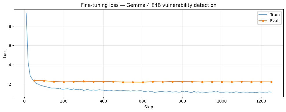
<p><img src="/images/gemma4-vuln/curves.png" alt="Training loss curve" />
<em>Fine-tuning loss curve. Training loss (blue) drops sharply from ~9.5 to ~1.3. Validation loss (orange) plateaus at ~2.3.</em></p>

<p><strong>Training loss</strong> dropped sharply from ~9.5 to ~1.3 in the first 100 steps. (A starting loss of ~9.5 is higher than typical text models — this is normal for Gemma 4’s multimodal architecture with its large vocabulary. The model hasn’t seen our task format before, so early predictions are essentially random across the full token space.) It continued declining gradually after that.</p>

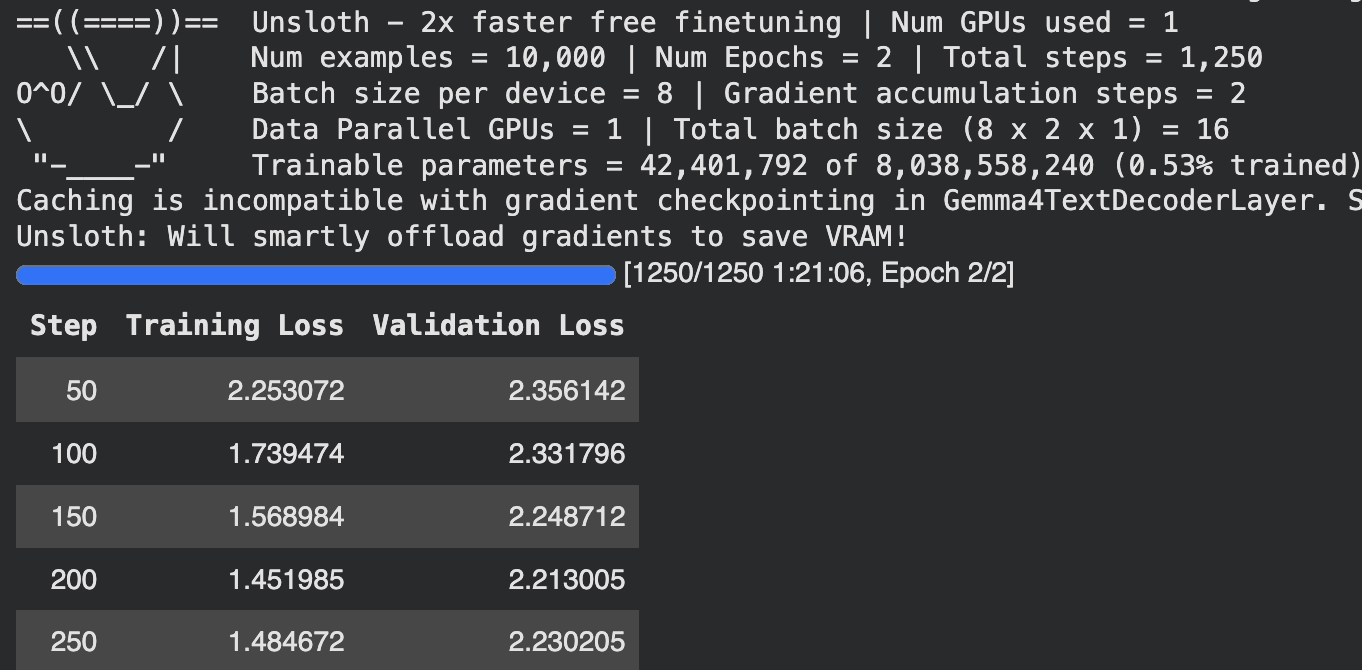
<p><strong>Validation loss</strong> dropped to ~2.3 and plateaued completely. Additional training steps reduced training loss but didn’t improve generalization. I had originally configured 3 epochs, but the validation curve made the decision clear: stop at 1 epoch. The model absorbed the clean, obvious patterns quickly. Further training was fitting the noisy labels, not learning new patterns.</p>

<p><img src="/images/gemma4-vuln/fine-tune-progress.png" alt="Unsloth training output" />
<em>Unsloth training progress — step-by-step loss showing the plateau during epoch 1.</em></p>

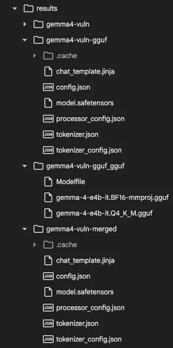
<p><img src="/images/gemma4-vuln/other-folders.jpeg" alt="Output files on Google Drive" />
<em>Three output formats saved to Google Drive — LoRA adapter, merged SafeTensors, and GGUF.</em></p>

<h2 id="the-fine-tuned-model-is-saved-in-three-formats">The fine-tuned model is saved in three formats…</h2>

<h2 id="evaluation-three-iterations-to-honest-numbers">Evaluation: three iterations to honest numbers</h2>

<p>Evaluating this model correctly turned out to be harder than training it.</p>

<svg width="100%" viewBox="0 0 680 160" xmlns="http://www.w3.org/2000/svg" style="max-width:680px;margin:1.5em auto;display:block">
  <style>text{font-family:-apple-system,BlinkMacSystemFont,"Segoe UI",sans-serif}</style>
  <rect x="0" y="0" width="680" height="160" rx="12" fill="#f9f9f7" stroke="#e5e4e0" stroke-width="1" />
  <text x="340" y="24" text-anchor="middle" font-size="12" font-weight="500" fill="#3d3d3a">Three iterations to honest numbers</text>
  <!-- Iteration 1 -->
  <rect x="30" y="44" width="180" height="72" rx="8" fill="#FCEBEB" stroke="#E24B4A" stroke-width="0.5" />
  <text x="120" y="66" text-anchor="middle" font-size="12" font-weight="600" fill="#791F1F">94.5% accuracy</text>
  <text x="120" y="82" text-anchor="middle" font-size="10" fill="#A32D2D">Imbalanced test set</text>
  <text x="120" y="96" text-anchor="middle" font-size="10" fill="#A32D2D">195 safe, 5 vulnerable</text>
  <text x="120" y="110" text-anchor="middle" font-size="9" font-style="italic" fill="#791F1F">Misleading ✗</text>
  <!-- Arrow -->
  <text x="232" y="82" text-anchor="middle" font-size="14" fill="#888">→</text>
  <!-- Iteration 2 -->
  <rect x="250" y="44" width="180" height="72" rx="8" fill="#FAEEDA" stroke="#BA7517" stroke-width="0.5" />
  <text x="340" y="66" text-anchor="middle" font-size="12" font-weight="600" fill="#633806">52.5% / 7% recall</text>
  <text x="340" y="82" text-anchor="middle" font-size="10" fill="#BA7517">Balanced, but prompt echo</text>
  <text x="340" y="96" text-anchor="middle" font-size="10" fill="#BA7517">Model parroting template</text>
  <text x="340" y="110" text-anchor="middle" font-size="9" font-style="italic" fill="#633806">Prompt bug ✗</text>
  <!-- Arrow -->
  <text x="452" y="82" text-anchor="middle" font-size="14" fill="#888">→</text>
  <!-- Iteration 3 -->
  <rect x="470" y="44" width="180" height="72" rx="8" fill="#E1F5EE" stroke="#1D9E75" stroke-width="0.5" />
  <text x="560" y="66" text-anchor="middle" font-size="12" font-weight="600" fill="#085041">61.0% / F1 0.567</text>
  <text x="560" y="82" text-anchor="middle" font-size="10" fill="#0F6E56">Balanced + fixed prompt</text>
  <text x="560" y="96" text-anchor="middle" font-size="10" fill="#0F6E56">51 of 100 vulns caught</text>
  <text x="560" y="110" text-anchor="middle" font-size="9" font-style="italic" fill="#085041">Real result ✓</text>
  <text x="340" y="146" text-anchor="middle" font-size="10" fill="#888780">Each iteration fixed the measurement, not the model — the weights never changed</text>
</svg>

<hr />

<h3 id="the-accuracy-trap">The accuracy trap</h3>

<p>First run on 200 random test samples: <strong>94.5% accuracy</strong>. Impressive — until you check the distribution. 195 safe, 5 vulnerable. The raw test set mirrors the original dataset’s 95/5 imbalance. The model said “SAFE” almost every time and scored well by default.</p>

<p><strong>Lesson:</strong> always evaluate on a balanced test set. Accuracy on imbalanced data is meaningless.</p>

<hr />

<h3 id="the-prompt-echo">The prompt echo</h3>

<p>Balanced evaluation (100 vulnerable + 100 safe): <strong>52.5% accuracy, 7% recall</strong>. Something was clearly wrong. I looked at the actual model outputs:</p>

<div class="language-plaintext highlighter-rouge"><div class="highlight"><pre class="highlight"><code>CWE: CWE-416
Model said: SAFE and a brief reason.

CWE: CWE-20, CWE-787
Model said: SAFE and a brief reason.
</code></pre></div></div>

<p>The model wasn’t analyzing code — it was <strong>echoing the prompt</strong>. The training data used the phrase “Reply with VULNERABLE or SAFE and a brief reason.” At inference time, the model encountered this substring and completed the most probable next tokens — which were the rest of the training template. This is a generation artifact: the model had learned the task, but the decoding followed a memorized path instead of producing new analysis.</p>

<p>The fix was simple: change the prompt wording at inference so it couldn’t trigger the memorized completion. Same model, same weights, different question:</p>

<div class="language-python highlighter-rouge"><div class="highlight"><pre class="highlight"><code><span class="c1"># Triggered memorized template completion
</span><span class="s">"Reply with VULNERABLE or SAFE and a brief reason."</span>

<span class="c1"># Fixed — new wording, model produces actual analysis
</span><span class="s">"Is it VULNERABLE or SAFE? Explain your reasoning."</span>
</code></pre></div></div>

<p>The model immediately started producing real analysis:</p>

<div class="language-plaintext highlighter-rouge"><div class="highlight"><pre class="highlight"><code>CWE: unknown
Model: This function is VULNERABLE. The function uses fork() to
execute a command in a child process...

CWE: CWE-190
Model: VULNERABLE. The function TIFFReadRawStrip1 is vulnerable
to a buffer overflow when reading raw data from a TIFF file...
</code></pre></div></div>

<p><strong>Lesson:</strong> fine-tuning teaches a conversational pattern, not just a task. The inference prompt must align with — but not exactly match — the training format. If the prompt contains a substring from training targets, the model may complete the template rather than reason about the input.</p>

<hr />

<h3 id="the-real-numbers">The real numbers</h3>

<p>Balanced evaluation, 200 samples (100 vulnerable + 100 safe), corrected prompt, with <code class="language-plaintext highlighter-rouge">random.seed(42)</code> for reproducibility. Both the fine-tuned and zero-shot models were evaluated with the identical prompt and the same 200 samples for a fair comparison:</p>

<table>
  <thead>
    <tr>
      <th> </th>
      <th>Fine-tuned</th>
      <th>Zero-shot (no training)</th>
      <th>Delta</th>
    </tr>
  </thead>
  <tbody>
    <tr>
      <td>Accuracy</td>
      <td>61.0%</td>
      <td>45.5%</td>
      <td>+15.5%</td>
    </tr>
    <tr>
      <td>Precision</td>
      <td>63.7%</td>
      <td>23.5%</td>
      <td>+40.2%</td>
    </tr>
    <tr>
      <td>Recall</td>
      <td>51.0%</td>
      <td>4.0%</td>
      <td>+47.0%</td>
    </tr>
    <tr>
      <td>F1</td>
      <td>0.567</td>
      <td>0.068</td>
      <td>+0.499</td>
    </tr>
  </tbody>
</table>

<p>The base Gemma 4 E4B caught 4 out of 100 vulnerabilities zero-shot — essentially guessing. The fine-tuned version caught 51, bringing recall from near-zero to about half. Not perfect, but a clear signal that the fine-tuning worked, especially given the noisy labels in the training data.</p>

<svg width="100%" viewBox="0 0 680 170" xmlns="http://www.w3.org/2000/svg" style="max-width:680px;margin:1.5em auto;display:block">
  <style>text{font-family:-apple-system,BlinkMacSystemFont,"Segoe UI",sans-serif}</style>
  <rect x="0" y="0" width="680" height="170" rx="12" fill="#f9f9f7" stroke="#e5e4e0" stroke-width="1" />
  <text x="340" y="24" text-anchor="middle" font-size="12" font-weight="500" fill="#3d3d3a">Recall comparison — how many vulnerabilities were caught out of 100</text>
  <!-- Zero-shot -->
  <text x="145" y="60" text-anchor="end" font-size="11" fill="#5F5E5A">Zero-shot (base)</text>
  <rect x="155" y="46" width="20" height="22" rx="3" fill="#FCEBEB" stroke="#E24B4A" stroke-width="0.5" />
  <text x="185" y="62" font-size="11" font-weight="500" fill="#791F1F">4 / 100</text>
  <!-- Fine-tuned -->
  <text x="145" y="100" text-anchor="end" font-size="11" fill="#5F5E5A">Fine-tuned (ours)</text>
  <rect x="155" y="86" width="255" height="22" rx="3" fill="#E1F5EE" stroke="#1D9E75" stroke-width="0.5" />
  <text x="420" y="102" font-size="11" font-weight="500" fill="#085041">51 / 100</text>
  <!-- Scale -->
  <line x1="155" y1="122" x2="655" y2="122" stroke="#e5e4e0" stroke-width="0.5" />
  <text x="155" y="140" font-size="9" fill="#888780">0</text>
  <text x="405" y="140" text-anchor="middle" font-size="9" fill="#888780">50</text>
  <text x="655" y="140" text-anchor="end" font-size="9" fill="#888780">100</text>
  <text x="340" y="160" text-anchor="middle" font-size="10" fill="#888780">Same 200 test samples · same prompt · random.seed(42)</text>
</svg>

<hr />

<h2 id="what-did-fine-tuning-actually-change">What did fine-tuning actually change?</h2>

<p>Here’s what’s counterintuitive: we didn’t teach Gemma 4 about vulnerabilities. It already knew. The model was pre-trained on code, security advisories, CWE descriptions, and countless discussions about buffer overflows and injection attacks. The zero-shot baseline proved this — it sometimes gave detailed, correct explanations of why code was dangerous.</p>

<p>But it only caught 4 out of 100 vulnerabilities in our eval. Why?</p>

<p>Because our eval looked for the word “VULNERABLE” in the response. The base model would say things like “this code has potential security implications that warrant further review” — technically correct analysis, but our parser reads that as SAFE because it doesn’t contain the keyword. A smarter parser that also caught phrases like “security flaw” or “dangerous” would have narrowed the gap — but the inconsistency and lack of structured verdicts would remain. The model knew the answer but expressed it in a way our system couldn’t reliably use.</p>

<p>Fine-tuning was essentially <strong>response format alignment</strong> — teaching the model to package what it already knew into the structured output we needed:</p>

<ol>
  <li><strong>Lead with a verdict</strong> — always say VULNERABLE or SAFE first, not a hedged paragraph</li>
  <li><strong>Be consistent</strong> — same format every time, not sometimes three paragraphs and sometimes one word</li>
  <li><strong>Commit to a decision</strong> — no “this could potentially be problematic” — yes or no</li>
</ol>

<p>Think of it as a senior security consultant who knows everything about vulnerabilities but has never used your team’s reporting template. They can write a brilliant analysis, but they can’t fill in the “Severity: HIGH/MEDIUM/LOW” field consistently. Fine-tuning taught the consultant to use the template.</p>

<p>This is an important insight for anyone considering fine-tuning: if the base model already understands your domain, you may not need thousands of examples to teach it new knowledge. You need enough examples to teach it your expected response structure. In our case, one epoch was sufficient — the model learned the format fast, because the underlying knowledge was already there.</p>

<hr />

<h2 id="what-it-catches-and-what-it-misses">What it catches and what it misses</h2>

<p>Running the fine-tuned model against 200 vulnerable test samples grouped by CWE reveals a clear pattern. A caveat: sample sizes per CWE are small (some have only 4 samples), so these recall numbers are indicative of trends, not statistically robust benchmarks.</p>

<p><strong>Strong performers (&gt;60% recall):</strong></p>

<table>
  <thead>
    <tr>
      <th>CWE</th>
      <th>Description</th>
      <th>Caught</th>
      <th>Total</th>
      <th>Recall</th>
    </tr>
  </thead>
  <tbody>
    <tr>
      <td>CWE-310</td>
      <td>Cryptographic issues</td>
      <td>3</td>
      <td>4</td>
      <td>75.0%</td>
    </tr>
    <tr>
      <td>CWE-20</td>
      <td>Input validation</td>
      <td>12</td>
      <td>17</td>
      <td>70.6%</td>
    </tr>
    <tr>
      <td>CWE-200</td>
      <td>Information exposure</td>
      <td>4</td>
      <td>6</td>
      <td>66.7%</td>
    </tr>
    <tr>
      <td>CWE-787</td>
      <td>Out-of-bounds write</td>
      <td>16</td>
      <td>25</td>
      <td>64.0%</td>
    </tr>
  </tbody>
</table>

<p><strong>Weak spots (&lt;35% recall):</strong></p>

<table>
  <thead>
    <tr>
      <th>CWE</th>
      <th>Description</th>
      <th>Caught</th>
      <th>Total</th>
      <th>Recall</th>
    </tr>
  </thead>
  <tbody>
    <tr>
      <td>CWE-415</td>
      <td>Double free</td>
      <td>0</td>
      <td>4</td>
      <td>0.0%</td>
    </tr>
    <tr>
      <td>CWE-401</td>
      <td>Memory leak</td>
      <td>1</td>
      <td>4</td>
      <td>25.0%</td>
    </tr>
    <tr>
      <td>CWE-399</td>
      <td>Resource management</td>
      <td>1</td>
      <td>4</td>
      <td>25.0%</td>
    </tr>
    <tr>
      <td>CWE-416</td>
      <td>Use after free</td>
      <td>4</td>
      <td>12</td>
      <td>33.3%</td>
    </tr>
  </tbody>
</table>

<svg width="100%" viewBox="0 0 680 310" xmlns="http://www.w3.org/2000/svg" style="max-width:680px;margin:1.5em auto;display:block">
  <style>text{font-family:-apple-system,BlinkMacSystemFont,"Segoe UI",sans-serif}</style>
  <rect x="0" y="0" width="680" height="310" rx="12" fill="#f9f9f7" stroke="#e5e4e0" stroke-width="1" />
  <text x="340" y="24" text-anchor="middle" font-size="12" font-weight="500" fill="#3d3d3a">Recall by CWE — what the model catches vs misses</text>
  <!-- CWE-310 75% -->
  <text x="155" y="52" text-anchor="end" font-size="10" fill="#5F5E5A">CWE-310 Crypto</text>
  <rect x="165" y="40" width="375" height="18" rx="3" fill="#E1F5EE" stroke="#1D9E75" stroke-width="0.5" />
  <text x="548" y="54" font-size="10" fill="#085041">75%</text>
  <!-- CWE-20 70.6% -->
  <text x="155" y="78" text-anchor="end" font-size="10" fill="#5F5E5A">CWE-20 Input val.</text>
  <rect x="165" y="66" width="353" height="18" rx="3" fill="#E1F5EE" stroke="#1D9E75" stroke-width="0.5" />
  <text x="526" y="80" font-size="10" fill="#085041">70.6%</text>
  <!-- CWE-200 66.7% -->
  <text x="155" y="104" text-anchor="end" font-size="10" fill="#5F5E5A">CWE-200 Info exp.</text>
  <rect x="165" y="92" width="333" height="18" rx="3" fill="#E1F5EE" stroke="#1D9E75" stroke-width="0.5" />
  <text x="506" y="106" font-size="10" fill="#085041">66.7%</text>
  <!-- CWE-787 64% -->
  <text x="155" y="130" text-anchor="end" font-size="10" fill="#5F5E5A">CWE-787 OOB write</text>
  <rect x="165" y="118" width="320" height="18" rx="3" fill="#E1F5EE" stroke="#1D9E75" stroke-width="0.5" />
  <text x="493" y="132" font-size="10" fill="#085041">64%</text>
  <!-- Divider -->
  <line x1="30" y1="150" x2="650" y2="150" stroke="#e5e4e0" stroke-width="0.5" stroke-dasharray="4 3" />
  <!-- CWE-476 55.6% -->
  <text x="155" y="174" text-anchor="end" font-size="10" fill="#5F5E5A">CWE-476 NULL deref</text>
  <rect x="165" y="162" width="278" height="18" rx="3" fill="#FAEEDA" stroke="#BA7517" stroke-width="0.5" />
  <text x="451" y="176" font-size="10" fill="#633806">55.6%</text>
  <!-- CWE-416 33.3% -->
  <text x="155" y="200" text-anchor="end" font-size="10" fill="#5F5E5A">CWE-416 Use after free</text>
  <rect x="165" y="188" width="167" height="18" rx="3" fill="#FCEBEB" stroke="#E24B4A" stroke-width="0.5" />
  <text x="340" y="202" font-size="10" fill="#791F1F">33.3%</text>
  <!-- CWE-401 25% -->
  <text x="155" y="226" text-anchor="end" font-size="10" fill="#5F5E5A">CWE-401 Mem leak</text>
  <rect x="165" y="214" width="125" height="18" rx="3" fill="#FCEBEB" stroke="#E24B4A" stroke-width="0.5" />
  <text x="298" y="228" font-size="10" fill="#791F1F">25%</text>
  <!-- CWE-415 0% -->
  <text x="155" y="252" text-anchor="end" font-size="10" fill="#5F5E5A">CWE-415 Double free</text>
  <rect x="165" y="240" width="3" height="18" rx="1" fill="#FCEBEB" stroke="#E24B4A" stroke-width="0.5" />
  <text x="178" y="254" font-size="10" fill="#791F1F">0%</text>
  <!-- Legend -->
  <rect x="165" y="278" width="12" height="12" rx="2" fill="#E1F5EE" stroke="#1D9E75" stroke-width="0.5" />
  <text x="183" y="289" font-size="9" fill="#5F5E5A">Pattern-based (localized signatures)</text>
  <rect x="380" y="278" width="12" height="12" rx="2" fill="#FCEBEB" stroke="#E24B4A" stroke-width="0.5" />
  <text x="398" y="289" font-size="9" fill="#5F5E5A">State-tracking (execution flow)</text>
</svg>

<p>The model catches vulnerabilities with obvious, localized code signatures — unchecked inputs, buffer writes without bounds checking, weak crypto usage. These are patterns where a single line or function call is the red flag.</p>

<p>Where it struggles is with <strong>state-tracking bugs</strong> — double frees, use-after-free, memory leaks. These vulnerabilities require understanding execution flow across multiple lines: memory was allocated here, freed there, and then accessed again somewhere else. A model looking at a single function in isolation has limited ability to track that kind of stateful reasoning.</p>

<p>Fine-tuning taught the model to recognize vulnerability <em>signatures</em>, not to perform deep program analysis. True flow-sensitive analysis would likely require either a much larger model, a multi-file context approach, or combining the LLM with static analysis tools — for example, using Semgrep or CodeQL to identify candidate functions, then the LLM to classify and explain. That hybrid approach is worth exploring in a future post.</p>

<hr />

<h2 id="key-takeaways">Key takeaways</h2>

<p><strong>Watch the validation loss, not the training loss.</strong> Training loss always keeps dropping — that’s memorization. Validation loss tells you when to stop. Mine plateaued halfway through epoch 1.</p>

<p><strong>Evaluation is harder than training.</strong> My reported accuracy changed from 94.5% to 52.5% to 61% across three iterations. Each time, the problem was measurement, not the model.</p>

<p><strong>Prompt alignment matters more than you’d expect.</strong> The model learned fine — but the inference prompt triggered a memorized template completion instead of actual analysis. Changing the prompt wording fixed it instantly, with no retraining.</p>

<p><strong>Data quality is the ceiling.</strong> With ~60% label accuracy (<a href="https://surrealyz.github.io/files/pubs/raid23-diversevul.pdf">DiverseVul, RAID 2023</a>), no training configuration will produce great results. For production, invest in labels first. For learning, noisy data teaches you the process just as well.</p>

<p><strong>Practical note:</strong> if you’re training on Google Colab, save to Google Drive early and often. I lost a full training run when the session disconnected. Mount Drive at the start and set your output directory there.</p>

<hr />

<h2 id="the-outputs">The outputs</h2>
<p><img src="/images/gemma4-vuln/other-folders.jpeg" alt="Outputs" /></p>

<p>The fine-tuned model is saved in three formats: a <strong>LoRA adapter</strong> (~160MB), a <strong>merged 16-bit SafeTensors</strong> model (~8GB), and a <strong>GGUF Q4_K_M</strong> file (~2.5GB). The evaluation in this post was done on the SafeTensors LoRA checkpoint. The GGUF version hasn’t been evaluated yet — that’s the focus of the next post.</p>

<hr />

<h2 id="whats-next">What’s next</h2>

<p>In the next post, I’ll take the GGUF file and benchmark different quantization levels — Q4 vs Q5 vs Q8 — measuring what you lose when you shrink a model from 8GB to 2.5GB. Does Q4 still catch the buffer overflows that Q8 catches? Where exactly is the quality cliff?</p>

<p>The code for the full experiment: <a href="https://github.com/Geo-Joy/llm-vuln-detector">https://github.com/Geo-Joy/llm-vuln-detector</a></p>

<hr />

<p><em>This is Part 1 of “The Security Engineer’s Practical Guide to LLMs.” Concepts reference: <strong><a href="/posts/every-concept-before-fine-tuning-llm/">Every Concept You Need Before Fine-Tuning an LLM</a></strong>. Next: What you lose when you shrink a model 4x.</em></p>]]></content><author><name>Geo Joy</name><email>breachguru@gmail.com</email></author><category term="LLM" /><category term="fine-tuning" /><category term="Gemma 4" /><category term="code security" /><category term="Unsloth" /><summary type="html"><![CDATA[One GPU, one epoch, three evaluation surprises, and recall that jumped from 4% to 51%. If you want the concepts behind the decisions (LoRA, QLoRA, NF4, batch size, loss curves), read the companion reference: Every Concept You Need Before Fine-Tuning an LLM.]]></summary></entry><entry><title type="html">Every Concept You Need Before Fine-Tuning an LLM</title><link href="https://breach.guru/posts/every-concept-before-fine-tuning-llm/" rel="alternate" type="text/html" title="Every Concept You Need Before Fine-Tuning an LLM" /><published>2026-05-01T00:00:00+00:00</published><updated>2026-05-01T00:00:00+00:00</updated><id>https://breach.guru/posts/every-concept-before-fine-tuning-llm</id><content type="html" xml:base="https://breach.guru/posts/every-concept-before-fine-tuning-llm/"><![CDATA[<p><em>A practitioner’s reference — LoRA, QLoRA, batch size, loss curves, and output formats explained. This is the concepts companion to <strong><a href="/posts/fine-tuned-gemma4-code-vulnerabilities/">I Fine-Tuned Gemma 4 to Detect Code Vulnerabilities — Here’s What Happened</a></strong>.</em></p>

<p><em>Most engineering teams use LLMs through APIs — prompt in, response out. The models themselves are a black box. Fine-tuning opens that box: instead of crafting better prompts, you adjust the model’s weights directly. I recently ran my first fine-tuning experiment and spent more time understanding the concepts than writing the code. This post is the reference guide I wish existed when I started.</em></p>

<svg width="100%" viewBox="0 0 680 310" xmlns="http://www.w3.org/2000/svg" style="max-width:680px;margin:1.5em auto;display:block">
  <style>text{font-family:-apple-system,BlinkMacSystemFont,"Segoe UI",sans-serif}</style>
  <rect x="0" y="0" width="680" height="310" rx="12" fill="#f9f9f7" stroke="#e5e4e0" stroke-width="1" />
  <defs><marker id="arr3" viewBox="0 0 10 10" refX="8" refY="5" markerWidth="6" markerHeight="6" orient="auto-start-reverse"><path d="M2 1L8 5L2 9" fill="none" stroke="context-stroke" stroke-width="1.5" stroke-linecap="round" stroke-linejoin="round" /></marker></defs>
  <text x="340" y="24" text-anchor="middle" font-size="13" font-weight="500" fill="#3d3d3a">The fine-tuning pipeline — where each concept fits</text>
  <!-- Stage 1: Setup -->
  <rect x="16" y="42" width="142" height="244" rx="10" fill="#fff" stroke="#e5e4e0" stroke-width="0.5" />
  <rect x="16" y="42" width="142" height="28" rx="10" fill="#EEEDFE" />
  <rect x="16" y="56" width="142" height="14" fill="#EEEDFE" />
  <text x="87" y="61" text-anchor="middle" font-size="11" font-weight="500" fill="#3C3489">1. Setup</text>
  <rect x="28" y="82" width="118" height="28" rx="4" fill="#EEEDFE" stroke="#B5ADF2" stroke-width="0.5" />
  <text x="87" y="100" text-anchor="middle" font-size="10" fill="#3C3489">SFT paradigm</text>
  <rect x="28" y="116" width="118" height="28" rx="4" fill="#EEEDFE" stroke="#B5ADF2" stroke-width="0.5" />
  <text x="87" y="134" text-anchor="middle" font-size="10" fill="#3C3489">Input/output pairs</text>
  <rect x="28" y="150" width="118" height="28" rx="4" fill="#EEEDFE" stroke="#B5ADF2" stroke-width="0.5" />
  <text x="87" y="168" text-anchor="middle" font-size="10" fill="#3C3489">Chat template</text>
  <!-- Arrow 1→2 -->
  <line x1="158" y1="164" x2="194" y2="164" stroke="#b4b2a9" stroke-width="0.5" marker-end="url(#arr3)" />
  <!-- Stage 2: Model Loading -->
  <rect x="198" y="42" width="160" height="244" rx="10" fill="#fff" stroke="#e5e4e0" stroke-width="0.5" />
  <rect x="198" y="42" width="160" height="28" rx="10" fill="#E6F1FB" />
  <rect x="198" y="56" width="160" height="14" fill="#E6F1FB" />
  <text x="278" y="61" text-anchor="middle" font-size="11" font-weight="500" fill="#0C447C">2. Load model</text>
  <rect x="210" y="82" width="136" height="28" rx="4" fill="#E6F1FB" stroke="#85B7EB" stroke-width="0.5" />
  <text x="278" y="100" text-anchor="middle" font-size="10" fill="#0C447C">LoRA adapters</text>
  <rect x="210" y="116" width="136" height="28" rx="4" fill="#E6F1FB" stroke="#85B7EB" stroke-width="0.5" />
  <text x="278" y="134" text-anchor="middle" font-size="10" fill="#0C447C">QLoRA (4-bit loading)</text>
  <rect x="210" y="150" width="136" height="28" rx="4" fill="#E6F1FB" stroke="#85B7EB" stroke-width="0.5" />
  <text x="278" y="168" text-anchor="middle" font-size="10" fill="#0C447C">NF4 quantization</text>
  <rect x="210" y="184" width="136" height="28" rx="4" fill="#E6F1FB" stroke="#85B7EB" stroke-width="0.5" />
  <text x="278" y="202" text-anchor="middle" font-size="10" fill="#0C447C">Gradient checkpointing</text>
  <!-- Arrow 2→3 -->
  <line x1="358" y1="164" x2="394" y2="164" stroke="#b4b2a9" stroke-width="0.5" marker-end="url(#arr3)" />
  <!-- Stage 3: Training -->
  <rect x="398" y="42" width="142" height="244" rx="10" fill="#fff" stroke="#e5e4e0" stroke-width="0.5" />
  <rect x="398" y="42" width="142" height="28" rx="10" fill="#FAEEDA" />
  <rect x="398" y="56" width="142" height="14" fill="#FAEEDA" />
  <text x="469" y="61" text-anchor="middle" font-size="11" font-weight="500" fill="#633806">3. Train</text>
  <rect x="410" y="82" width="118" height="28" rx="4" fill="#FAEEDA" stroke="#DEA544" stroke-width="0.5" />
  <text x="469" y="100" text-anchor="middle" font-size="10" fill="#633806">Batch size</text>
  <rect x="410" y="116" width="118" height="28" rx="4" fill="#FAEEDA" stroke="#DEA544" stroke-width="0.5" />
  <text x="469" y="134" text-anchor="middle" font-size="10" fill="#633806">Grad accumulation</text>
  <rect x="410" y="150" width="118" height="28" rx="4" fill="#FAEEDA" stroke="#DEA544" stroke-width="0.5" />
  <text x="469" y="168" text-anchor="middle" font-size="10" fill="#633806">Loss curves</text>
  <rect x="410" y="184" width="118" height="28" rx="4" fill="#FAEEDA" stroke="#DEA544" stroke-width="0.5" />
  <text x="469" y="202" text-anchor="middle" font-size="10" fill="#633806">Epochs</text>
  <!-- Arrow 3→4 -->
  <line x1="540" y1="164" x2="576" y2="164" stroke="#b4b2a9" stroke-width="0.5" marker-end="url(#arr3)" />
  <!-- Stage 4: Output -->
  <rect x="580" y="42" width="84" height="244" rx="10" fill="#fff" stroke="#e5e4e0" stroke-width="0.5" />
  <rect x="580" y="42" width="84" height="28" rx="10" fill="#E1F5EE" />
  <rect x="580" y="56" width="84" height="14" fill="#E1F5EE" />
  <text x="622" y="61" text-anchor="middle" font-size="11" font-weight="500" fill="#085041">4. Save</text>
  <rect x="590" y="82" width="64" height="28" rx="4" fill="#E1F5EE" stroke="#6BC8A8" stroke-width="0.5" />
  <text x="622" y="100" text-anchor="middle" font-size="10" fill="#085041">Adapter</text>
  <rect x="590" y="116" width="64" height="28" rx="4" fill="#E1F5EE" stroke="#6BC8A8" stroke-width="0.5" />
  <text x="622" y="134" text-anchor="middle" font-size="10" fill="#085041">Merged</text>
  <rect x="590" y="150" width="64" height="28" rx="4" fill="#E1F5EE" stroke="#6BC8A8" stroke-width="0.5" />
  <text x="622" y="168" text-anchor="middle" font-size="10" fill="#085041">GGUF</text>
  <!-- Memory note at bottom -->
  <rect x="16" y="296" width="648" height="1" fill="none" />
  <text x="340" y="306" text-anchor="middle" font-size="10" fill="#888780">Read left to right — each stage introduces the concepts explained in detail below.</text>
</svg>

<hr />

<h2 id="what-is-fine-tuning-and-why-not-just-prompt-better">What is fine-tuning, and why not just prompt better?</h2>

<p>Zero-shot prompting means giving an LLM instructions and hoping it follows them. It works surprisingly well for general tasks. But when you need a model to perform one specific task consistently — same format, same decision boundary, every time — fine-tuning has an edge.</p>

<p>You show the model thousands of input/output examples, and it adjusts its internal weights to reproduce that pattern. The result is a smaller, specialized model that does one thing reliably, versus a large general model that needs careful prompting and still varies.</p>

<hr />

<h2 id="whats-sft">What’s SFT?</h2>

<p><strong>SFT</strong> stands for <strong>Supervised Fine-Tuning</strong>. “Supervised” means you provide the right answers — input/output pairs. The model sees a code snippet (input) and the correct verdict like “VULNERABLE — CWE-120” (output), repeated thousands of times. It adjusts its weights to predict similar outputs for similar inputs.</p>

<p>This is different from <strong>RLHF</strong> (reinforcement learning from human feedback), where the model gets a score for how good its answer was, or unsupervised pre-training where the model just reads text with no labels. The <strong>SFTTrainer</strong> from the <strong>TRL</strong> (Transformer Reinforcement Learning) library — HuggingFace’s toolkit for fine-tuning and aligning LLMs — handles the mechanics: tokenization, masking user messages so the model only learns to predict assistant responses, and running the training loop.</p>

<p><strong>When to use SFT vs alternatives:</strong> SFT is the right choice when you have labeled data (input/output pairs) and want the model to produce structured, explainable responses. If you only needed a binary score without explanations, a <strong>classification head</strong> on top of the model would be simpler — though in my experiment I chose SFT because I wanted the model to also produce reasoning and CWE classifications alongside the verdict, not just a bare label. If you wanted to refine response <em>quality</em> after SFT, <strong>DPO</strong> (Direct Preference Optimization) takes pairs of good/bad responses and teaches the model to prefer the better one — that’s the SFT → DPO pipeline most production models use. <strong>RLHF</strong> goes further with a full reward model and reinforcement learning, but that’s overkill unless “good” is subjective and hard to label. For most fine-tuning projects, SFT is where you start.</p>

<hr />

<h2 id="what-are-lora-and-qlora">What are LoRA and QLoRA?</h2>

<p>Full fine-tuning updates all of a model’s parameters. For a model like Gemma 4 E4B, that’s 8 billion numbers — you’d need 80–100GB of GPU memory. The breakdown: 16GB for weights in 16-bit. 16GB for <strong>gradients</strong> — a value per weight that tells the optimizer <em>which direction and how steeply</em> the loss changes with respect to that weight. The optimizer then decides how far to actually move. 64GB for Adam optimizer states (it tracks momentum and variance for every weight, both in 32-bit). Plus activations. Even with memory-efficient optimizers, you’re looking at 60GB minimum. Not practical on most hardware.</p>

<svg width="100%" viewBox="0 0 680 310" xmlns="http://www.w3.org/2000/svg" style="max-width:680px;margin:1.5em auto;display:block">
  <style>text{font-family:-apple-system,BlinkMacSystemFont,"Segoe UI",sans-serif}</style>
  <rect x="0" y="0" width="680" height="310" rx="12" fill="#f9f9f7" stroke="#e5e4e0" stroke-width="1" />
  <text x="340" y="24" text-anchor="middle" font-size="13" font-weight="500" fill="#3d3d3a">Three ways to fine-tune — Full FT vs LoRA vs QLoRA</text>
  <!-- === Full Fine-Tuning === -->
  <rect x="22" y="40" width="200" height="250" rx="10" fill="#fff" stroke="#e5e4e0" stroke-width="0.5" />
  <rect x="22" y="40" width="200" height="30" rx="10" fill="#FCEBEB" />
  <rect x="22" y="56" width="200" height="14" fill="#FCEBEB" />
  <text x="122" y="60" text-anchor="middle" font-size="12" font-weight="500" fill="#791F1F">Full Fine-Tuning</text>
  <!-- Model blocks - all trainable -->
  <rect x="46" y="82" width="152" height="22" rx="4" fill="#FCEBEB" stroke="#E24B4A" stroke-width="0.5" />
  <text x="122" y="97" text-anchor="middle" font-size="10" fill="#A32D2D">Attention × 42</text>
  <rect x="46" y="110" width="152" height="22" rx="4" fill="#FCEBEB" stroke="#E24B4A" stroke-width="0.5" />
  <text x="122" y="125" text-anchor="middle" font-size="10" fill="#A32D2D">MLP × 42</text>
  <rect x="46" y="138" width="152" height="22" rx="4" fill="#FCEBEB" stroke="#E24B4A" stroke-width="0.5" />
  <text x="122" y="153" text-anchor="middle" font-size="10" fill="#A32D2D">Embeddings</text>
  <!-- Memory bar -->
  <rect x="46" y="178" width="152" height="44" rx="6" fill="#FCEBEB" stroke="#E24B4A" stroke-width="0.8" />
  <text x="122" y="196" text-anchor="middle" font-size="10" font-weight="500" fill="#791F1F">8B params trainable</text>
  <text x="122" y="212" text-anchor="middle" font-size="9" fill="#A32D2D">Weights + grads + optim</text>
  <text x="122" y="240" text-anchor="middle" font-size="12" font-weight="500" fill="#A32D2D">~100 GB</text>
  <!-- Arrow -->
  <text x="233" y="165" text-anchor="middle" font-size="18" fill="#b4b2a9">→</text>
  <!-- === LoRA === -->
  <rect x="244" y="40" width="200" height="250" rx="10" fill="#fff" stroke="#e5e4e0" stroke-width="0.5" />
  <rect x="244" y="40" width="200" height="30" rx="10" fill="#E6F1FB" />
  <rect x="244" y="56" width="200" height="14" fill="#E6F1FB" />
  <text x="344" y="60" text-anchor="middle" font-size="12" font-weight="500" fill="#0C447C">LoRA</text>
  <!-- Base model blocks - frozen -->
  <rect x="266" y="82" width="110" height="22" rx="4" fill="#fff" stroke="#B4B2A9" stroke-width="0.5" />
  <text x="321" y="97" text-anchor="middle" font-size="10" fill="#5F5E5A">Attn (frozen)</text>
  <!-- LoRA adapter blocks -->
  <rect x="382" y="82" width="42" height="22" rx="4" fill="#E1F5EE" stroke="#1D9E75" stroke-width="0.5" />
  <text x="403" y="97" text-anchor="middle" font-size="9" fill="#085041">+A</text>
  <rect x="266" y="110" width="110" height="22" rx="4" fill="#fff" stroke="#B4B2A9" stroke-width="0.5" />
  <text x="321" y="125" text-anchor="middle" font-size="10" fill="#5F5E5A">MLP (frozen)</text>
  <rect x="382" y="110" width="42" height="22" rx="4" fill="#E1F5EE" stroke="#1D9E75" stroke-width="0.5" />
  <text x="403" y="125" text-anchor="middle" font-size="9" fill="#085041">+A</text>
  <rect x="266" y="138" width="110" height="22" rx="4" fill="#fff" stroke="#B4B2A9" stroke-width="0.5" />
  <text x="321" y="153" text-anchor="middle" font-size="10" fill="#5F5E5A">Emb (frozen)</text>
  <!-- Memory bar -->
  <rect x="266" y="178" width="158" height="44" rx="6" fill="#E1F5EE" stroke="#1D9E75" stroke-width="0.8" />
  <text x="345" y="196" text-anchor="middle" font-size="10" font-weight="500" fill="#085041">42M params trainable</text>
  <text x="345" y="212" text-anchor="middle" font-size="9" fill="#0F6E56">Base frozen in 16-bit</text>
  <text x="345" y="240" text-anchor="middle" font-size="12" font-weight="500" fill="#0F6E56">~18 GB</text>
  <!-- Arrow -->
  <text x="455" y="165" text-anchor="middle" font-size="18" fill="#b4b2a9">→</text>
  <!-- === QLoRA === -->
  <rect x="466" y="40" width="192" height="250" rx="10" fill="#fff" stroke="#e5e4e0" stroke-width="0.5" />
  <rect x="466" y="40" width="192" height="30" rx="10" fill="#E1F5EE" />
  <rect x="466" y="56" width="192" height="14" fill="#E1F5EE" />
  <text x="562" y="60" text-anchor="middle" font-size="12" font-weight="500" fill="#085041">QLoRA</text>
  <!-- Base model blocks - frozen + compressed -->
  <rect x="486" y="82" width="94" height="22" rx="4" fill="#fff" stroke="#B4B2A9" stroke-width="0.5" stroke-dasharray="4 2" />
  <text x="533" y="97" text-anchor="middle" font-size="10" fill="#888780">Attn (4-bit)</text>
  <rect x="586" y="82" width="52" height="22" rx="4" fill="#E1F5EE" stroke="#1D9E75" stroke-width="0.5" />
  <text x="612" y="97" text-anchor="middle" font-size="9" fill="#085041">+A</text>
  <rect x="486" y="110" width="94" height="22" rx="4" fill="#fff" stroke="#B4B2A9" stroke-width="0.5" stroke-dasharray="4 2" />
  <text x="533" y="125" text-anchor="middle" font-size="10" fill="#888780">MLP (4-bit)</text>
  <rect x="586" y="110" width="52" height="22" rx="4" fill="#E1F5EE" stroke="#1D9E75" stroke-width="0.5" />
  <text x="612" y="125" text-anchor="middle" font-size="9" fill="#085041">+A</text>
  <rect x="486" y="138" width="94" height="22" rx="4" fill="#fff" stroke="#B4B2A9" stroke-width="0.5" stroke-dasharray="4 2" />
  <text x="533" y="153" text-anchor="middle" font-size="10" fill="#888780">Emb (4-bit)</text>
  <!-- Memory bar -->
  <rect x="486" y="178" width="152" height="44" rx="6" fill="#E1F5EE" stroke="#1D9E75" stroke-width="0.8" />
  <text x="562" y="196" text-anchor="middle" font-size="10" font-weight="500" fill="#085041">42M params trainable</text>
  <text x="562" y="212" text-anchor="middle" font-size="9" fill="#0F6E56">Base compressed to 4-bit NF4</text>
  <text x="562" y="240" text-anchor="middle" font-size="12" font-weight="500" fill="#0F6E56">~10 GB</text>
  <!-- Connecting note at bottom -->
  <text x="340" y="275" text-anchor="middle" font-size="10" fill="#5F5E5A">LoRA → QLoRA: the only change is compressing the frozen base from 16-bit to 4-bit.</text>
  <line x1="200" y1="290" x2="480" y2="290" stroke="#b4b2a9" stroke-width="0.5" />
  <text x="340" y="302" text-anchor="middle" font-size="10" fill="#888780">Same adapters, same training math, same gradients. Only the base model's storage format differs.</text>
</svg>

<p><strong>LoRA</strong> (Low-Rank Adaptation) takes a different approach. You freeze the entire base model and inject small trainable matrices into specific layers. These are called <strong>adapters</strong>. Think of it as: you have a textbook (the base model). Instead of rewriting every page, you add sticky notes to the pages that matter. The textbook stays the same; the sticky notes customize it for your task.</p>

<p>In my experiment, I trained 42 million parameters out of 8 billion — just 0.53% of the model. Where does that number come from? For each target layer, LoRA adds two small matrices instead of updating the full weight matrix. Say an attention layer has a weight matrix of size 3072 × 3072 (~9.4 million parameters). LoRA replaces that with two tiny matrices:</p>

<div class="language-plaintext highlighter-rouge"><div class="highlight"><pre class="highlight"><code>Original weight:  3072 × 3072 = 9,437,184 parameters
LoRA adapter A:   16 × 3072   = 49,152 parameters
LoRA adapter B:   3072 × 16   = 49,152 parameters
Total per module: 98,304 parameters (vs 9.4 million)
</code></pre></div></div>

<p>The <code class="language-plaintext highlighter-rouge">16</code> is the LoRA rank — our chosen adapter size. Multiply across 7 target modules (q, k, v, o, gate, up, down) per layer, across all 42 transformer layers, and you get ~42 million trainable parameters. Increase the rank to 32 and it doubles to ~84M. Drop to rank 8 and it halves to ~21M. The rank is your dial between “learn more” and “use less memory.”</p>

<svg width="100%" viewBox="0 0 680 270" xmlns="http://www.w3.org/2000/svg" style="max-width:680px;margin:1.5em auto;display:block">
  <style>text{font-family:-apple-system,BlinkMacSystemFont,"Segoe UI",sans-serif}</style>
  <rect x="0" y="0" width="680" height="270" rx="12" fill="#f9f9f7" stroke="#e5e4e0" stroke-width="1" />
  <text x="340" y="30" text-anchor="middle" font-size="13" font-weight="500" fill="#3d3d3a">LoRA rank decomposition — Gemma 4 E4B attention layer</text>
  <rect x="40" y="54" width="140" height="140" rx="4" fill="#FCEBEB" stroke="#A32D2D" stroke-width="0.5" />
  <text x="110" y="119" text-anchor="middle" font-size="13" font-weight="500" fill="#791F1F">Original W</text>
  <text x="110" y="139" text-anchor="middle" font-size="11" fill="#A32D2D">3072 × 3072</text>
  <text x="110" y="214" text-anchor="middle" font-size="11" fill="#791F1F">9.4M params</text>
  <text x="110" y="230" text-anchor="middle" font-size="11" fill="#A32D2D">All trainable</text>
  <text x="225" y="129" text-anchor="middle" font-size="18" fill="#888">→</text>
  <rect x="270" y="54" width="80" height="140" rx="4" fill="#E1F5EE" stroke="#0F6E56" stroke-width="0.5" />
  <text x="310" y="119" text-anchor="middle" font-size="13" font-weight="500" fill="#085041">B</text>
  <text x="310" y="139" text-anchor="middle" font-size="11" fill="#0F6E56">3072 × 16</text>
  <text x="375" y="129" text-anchor="middle" font-size="14" fill="#888">×</text>
  <rect x="400" y="99" width="140" height="44" rx="4" fill="#E1F5EE" stroke="#0F6E56" stroke-width="0.5" />
  <text x="470" y="117" text-anchor="middle" font-size="13" font-weight="500" fill="#085041">A</text>
  <text x="470" y="135" text-anchor="middle" font-size="11" fill="#0F6E56">16 × 3072</text>
  <text x="390" y="214" text-anchor="middle" font-size="11" fill="#085041">98K params (96× smaller)</text>
  <text x="390" y="230" text-anchor="middle" font-size="11" fill="#0F6E56">Only these train</text>
  <text x="340" y="258" text-anchor="middle" font-size="11" fill="#5F5E5A">× 7 modules × 42 layers = ~42M trainable (0.53% of Gemma 4 E4B)</text>
</svg>

<p>Because the base model is frozen, gradients and optimizer states are only computed for the adapter — 42 million parameters, not 8 billion. That’s why the memory drops dramatically.</p>

<p>The frozen base model still sits in GPU memory though. With standard LoRA, it stays at full 16-bit precision — that’s ~8GB just for weights you’re not even changing. That’s where QLoRA comes in.</p>

<p><strong>QLoRA</strong> is LoRA with exactly one change: compress the frozen base model to 4-bit when loading it into memory. The adapters, the training loop, the gradients, the optimizer — all identical to LoRA. The only difference is how much space the frozen base occupies in VRAM. In code, it’s a single flag: <code class="language-plaintext highlighter-rouge">load_in_4bit=True</code>. Set it to <code class="language-plaintext highlighter-rouge">False</code> and you’re doing standard LoRA. Set it to <code class="language-plaintext highlighter-rouge">True</code> and you’re doing QLoRA.</p>

<p>But that one flag triggers more than simple compression. Under the hood, the <strong>bitsandbytes</strong> library applies several innovations from the <a href="https://arxiv.org/abs/2305.14314">QLoRA paper</a> (Dettmers et al., 2023). The key one: it uses a smart compression method called <strong>NF4</strong> that’s specifically designed for neural network weights — instead of rounding numbers uniformly (which loses a lot), it places the 4-bit quantization levels where the weight values are most dense. This preserves 95–98% of model quality despite the 4x compression.</p>

<p>To be explicit: the adapters you’re training still run in full 16-bit precision — only the frozen base gets compressed. The base weights shrink from ~8GB to ~2.5GB, and the total setup fits comfortably on a single GPU. Everything else — LoRA rank, target modules, learning rate, batch size, gradient flow — stays the same.</p>

<p>Here’s the memory contrast:</p>

<table>
  <thead>
    <tr>
      <th> </th>
      <th>Full fine-tuning</th>
      <th>LoRA</th>
      <th>QLoRA</th>
    </tr>
  </thead>
  <tbody>
    <tr>
      <td>Base weights</td>
      <td>16GB (8B × 16-bit)</td>
      <td>16GB (8B × 16-bit, frozen)</td>
      <td><strong>2.5GB</strong> (8B × 4-bit, frozen)</td>
    </tr>
    <tr>
      <td>Gradients</td>
      <td>16GB (8B params)</td>
      <td>84MB (42M adapter params)</td>
      <td><strong>84MB</strong> (42M adapter params)</td>
    </tr>
    <tr>
      <td>Optimizer states</td>
      <td>64GB (8B × 2 × 32-bit)</td>
      <td>336MB (42M × 2 × 32-bit)</td>
      <td><strong>336MB</strong> (42M × 2 × 32-bit)</td>
    </tr>
    <tr>
      <td>Total (+ activations)</td>
      <td><strong>~100GB</strong></td>
      <td><strong>~18GB</strong></td>
      <td><strong>~10GB</strong></td>
    </tr>
  </tbody>
</table>

<p>Notice that LoRA and QLoRA have identical adapter sizes, gradient sizes, and optimizer sizes. The only row that changes is base weights — 16GB vs 2.5GB. That’s the entire difference.</p>

<p>Naive 4-bit compression would lose meaningful quality. NF4 is what makes QLoRA work — it’s the reason that one flag doesn’t tank your results.</p>

<svg width="100%" viewBox="0 0 680 410" xmlns="http://www.w3.org/2000/svg" style="max-width:680px;margin:1.5em auto;display:block">
  <style>text{font-family:-apple-system,BlinkMacSystemFont,"Segoe UI",sans-serif}</style>
  <rect x="0" y="0" width="680" height="410" rx="12" fill="#f9f9f7" stroke="#e5e4e0" stroke-width="1" />
  <text x="170" y="28" text-anchor="middle" font-size="13" font-weight="500" fill="#3d3d3a">Full fine-tuning</text>
  <text x="510" y="28" text-anchor="middle" font-size="13" font-weight="500" fill="#3d3d3a">QLoRA (what we used)</text>
  <!-- Left: full fine-tuning -->
  <rect x="60" y="48" width="220" height="290" rx="14" fill="#F1EFE8" stroke="#B4B2A9" stroke-width="0.5" />
  <text x="170" y="74" text-anchor="middle" font-size="12" font-weight="500" fill="#444441">Gemma 4 E4B — 8B params</text>
  <text x="170" y="90" text-anchor="middle" font-size="11" fill="#888780">All in 16-bit, all trainable</text>
  <rect x="80" y="106" width="180" height="36" rx="6" fill="#FCEBEB" stroke="#E24B4A" stroke-width="0.5" />
  <text x="170" y="128" text-anchor="middle" font-size="11" font-weight="500" fill="#791F1F">Attention × 42 layers</text>
  <rect x="80" y="152" width="180" height="36" rx="6" fill="#FCEBEB" stroke="#E24B4A" stroke-width="0.5" />
  <text x="170" y="174" text-anchor="middle" font-size="11" font-weight="500" fill="#791F1F">MLP × 42 layers</text>
  <rect x="80" y="198" width="180" height="36" rx="6" fill="#FCEBEB" stroke="#E24B4A" stroke-width="0.5" />
  <text x="170" y="220" text-anchor="middle" font-size="11" font-weight="500" fill="#791F1F">Embeddings (PLE)</text>
  <text x="170" y="264" text-anchor="middle" font-size="11" fill="#791F1F">Every weight updated</text>
  <text x="170" y="282" text-anchor="middle" font-size="12" font-weight="500" fill="#A32D2D">~100 GB needed</text>
  <text x="170" y="354" text-anchor="middle" font-size="11" fill="#888780">Weights: 16 GB</text>
  <text x="170" y="370" text-anchor="middle" font-size="11" fill="#888780">Gradients: 16 GB</text>
  <text x="170" y="386" text-anchor="middle" font-size="11" fill="#888780">Optimizer: 64 GB</text>
  <!-- Right: QLoRA -->
  <rect x="400" y="48" width="220" height="290" rx="14" fill="#E6F1FB" stroke="#85B7EB" stroke-width="0.5" />
  <text x="510" y="74" text-anchor="middle" font-size="12" font-weight="500" fill="#0C447C">Gemma 4 E4B — 8B params</text>
  <text x="510" y="90" text-anchor="middle" font-size="11" fill="#378ADD">Frozen in 4-bit NF4</text>
  <rect x="420" y="106" width="128" height="36" rx="6" fill="#fff" stroke="#B4B2A9" stroke-width="0.5" />
  <text x="484" y="128" text-anchor="middle" font-size="10" fill="#5F5E5A">Attention (frozen)</text>
  <rect x="554" y="106" width="52" height="36" rx="6" fill="#E1F5EE" stroke="#1D9E75" stroke-width="0.5" />
  <text x="580" y="128" text-anchor="middle" font-size="10" font-weight="500" fill="#085041">LoRA</text>
  <rect x="420" y="152" width="128" height="36" rx="6" fill="#fff" stroke="#B4B2A9" stroke-width="0.5" />
  <text x="484" y="174" text-anchor="middle" font-size="10" fill="#5F5E5A">MLP (frozen)</text>
  <rect x="554" y="152" width="52" height="36" rx="6" fill="#E1F5EE" stroke="#1D9E75" stroke-width="0.5" />
  <text x="580" y="174" text-anchor="middle" font-size="10" font-weight="500" fill="#085041">LoRA</text>
  <rect x="420" y="198" width="128" height="36" rx="6" fill="#fff" stroke="#B4B2A9" stroke-width="0.5" />
  <text x="484" y="220" text-anchor="middle" font-size="10" fill="#5F5E5A">Embeddings (frozen)</text>
  <text x="510" y="264" text-anchor="middle" font-size="11" fill="#085041">Only LoRA adapters train (0.53%)</text>
  <text x="510" y="282" text-anchor="middle" font-size="12" font-weight="500" fill="#0F6E56">~10 GB needed</text>
  <text x="510" y="354" text-anchor="middle" font-size="11" fill="#888780">Base weights: 2.5 GB (4-bit)</text>
  <text x="510" y="370" text-anchor="middle" font-size="11" fill="#888780">Adapter + grads: 168 MB</text>
  <text x="510" y="386" text-anchor="middle" font-size="11" fill="#888780">Optimizer: 336 MB</text>
  <!-- vs -->
  <text x="340" y="189" text-anchor="middle" font-size="13" fill="#888780">vs</text>
</svg>

<hr />

<h2 id="why-load-the-model-in-4-bit-wont-that-hurt-accuracy">Why load the model in 4-bit? Won’t that hurt accuracy?</h2>

<p>A model’s weights are just numbers — millions of them. Each number can be stored at different precisions:</p>

<ul>
  <li><strong>16-bit:</strong> high precision, like <code class="language-plaintext highlighter-rouge">3.141592653589793</code>. Takes more space.</li>
  <li><strong>4-bit:</strong> lower precision, like <code class="language-plaintext highlighter-rouge">3.1</code>. Takes 4x less space.</li>
</ul>

<p>The intuition says 4-bit should be much worse. And with naive rounding, it would be. But NF4 (the smart compression method used by QLoRA) places quantization levels where the weight values actually cluster rather than spacing them evenly. That’s why the research shows 95–98% quality retention.</p>

<svg width="100%" viewBox="0 0 680 420" xmlns="http://www.w3.org/2000/svg" style="max-width:680px;margin:1.5em auto;display:block">
  <style>text{font-family:-apple-system,BlinkMacSystemFont,"Segoe UI",sans-serif}</style>
  <rect x="0" y="0" width="680" height="420" rx="12" fill="#f9f9f7" stroke="#e5e4e0" stroke-width="1" />
  <text x="340" y="26" text-anchor="middle" font-size="13" font-weight="500" fill="#3d3d3a">Why NF4 beats naive 4-bit compression</text>
  <text x="340" y="42" text-anchor="middle" font-size="11" fill="#888780">Neural network weights follow a bell curve — most values cluster near zero.</text>
  <!-- === Top panel: Uniform 4-bit === -->
  <rect x="20" y="58" width="640" height="158" rx="10" fill="#fff" stroke="#e5e4e0" stroke-width="0.5" />
  <text x="340" y="80" text-anchor="middle" font-size="12" font-weight="500" fill="#A32D2D">Uniform 4-bit (naive rounding)</text>
  <text x="340" y="96" text-anchor="middle" font-size="10" fill="#888780">16 evenly spaced levels across the full range</text>
  <!-- Bell curve -->
  <path d="M 90,186 C 140,186 186,140 230,92 C 260,60 296,44 340,40 C 384,44 420,60 450,92 C 494,140 540,186 590,186" fill="#FCEBEB" fill-opacity="0.5" stroke="#E24B4A" stroke-width="0.8" />
  <!-- X-axis line -->
  <line x1="90" y1="186" x2="590" y2="186" stroke="#d4d3cf" stroke-width="0.5" />
  <!-- Uniform tick marks (16 evenly spaced) -->
  <line x1="90" y1="186" x2="90" y2="196" stroke="#A32D2D" stroke-width="0.8" />
  <line x1="106" y1="186" x2="106" y2="196" stroke="#A32D2D" stroke-width="0.8" />
  <line x1="139" y1="186" x2="139" y2="196" stroke="#A32D2D" stroke-width="0.8" />
  <line x1="172" y1="186" x2="172" y2="196" stroke="#A32D2D" stroke-width="0.8" />
  <line x1="206" y1="186" x2="206" y2="196" stroke="#A32D2D" stroke-width="0.8" />
  <line x1="239" y1="186" x2="239" y2="196" stroke="#A32D2D" stroke-width="0.8" />
  <line x1="272" y1="186" x2="272" y2="196" stroke="#A32D2D" stroke-width="0.8" />
  <line x1="306" y1="186" x2="306" y2="196" stroke="#A32D2D" stroke-width="0.8" />
  <line x1="340" y1="186" x2="340" y2="196" stroke="#A32D2D" stroke-width="0.8" />
  <line x1="374" y1="186" x2="374" y2="196" stroke="#A32D2D" stroke-width="0.8" />
  <line x1="408" y1="186" x2="408" y2="196" stroke="#A32D2D" stroke-width="0.8" />
  <line x1="441" y1="186" x2="441" y2="196" stroke="#A32D2D" stroke-width="0.8" />
  <line x1="474" y1="186" x2="474" y2="196" stroke="#A32D2D" stroke-width="0.8" />
  <line x1="508" y1="186" x2="508" y2="196" stroke="#A32D2D" stroke-width="0.8" />
  <line x1="541" y1="186" x2="541" y2="196" stroke="#A32D2D" stroke-width="0.8" />
  <line x1="574" y1="186" x2="574" y2="196" stroke="#A32D2D" stroke-width="0.8" />
  <!-- Wasted annotation brackets -->
  <line x1="90" y1="200" x2="90" y2="208" stroke="#A32D2D" stroke-width="0.5" />
  <line x1="206" y1="200" x2="206" y2="208" stroke="#A32D2D" stroke-width="0.5" />
  <line x1="90" y1="204" x2="206" y2="204" stroke="#A32D2D" stroke-width="0.5" stroke-dasharray="3 2" />
  <text x="148" y="218" text-anchor="middle" font-size="9" fill="#A32D2D">~6 levels wasted on near-empty tails</text>
  <!-- === Bottom panel: NF4 === -->
  <rect x="20" y="236" width="640" height="158" rx="10" fill="#fff" stroke="#e5e4e0" stroke-width="0.5" />
  <text x="340" y="258" text-anchor="middle" font-size="12" font-weight="500" fill="#0F6E56">NF4 (QLoRA's method)</text>
  <text x="340" y="274" text-anchor="middle" font-size="10" fill="#888780">16 levels placed at quantiles of the normal distribution — dense where weights are dense</text>
  <!-- Same bell curve -->
  <path d="M 90,364 C 140,364 186,318 230,270 C 260,238 296,222 340,218 C 384,222 420,238 450,270 C 494,318 540,364 590,364" fill="#E1F5EE" fill-opacity="0.5" stroke="#1D9E75" stroke-width="0.8" />
  <line x1="90" y1="364" x2="590" y2="364" stroke="#d4d3cf" stroke-width="0.5" />
  <!-- NF4 tick marks (clustered near center) -->
  <line x1="194" y1="364" x2="194" y2="374" stroke="#0F6E56" stroke-width="0.8" />
  <line x1="218" y1="364" x2="218" y2="374" stroke="#0F6E56" stroke-width="0.8" />
  <line x1="238" y1="364" x2="238" y2="374" stroke="#0F6E56" stroke-width="0.8" />
  <line x1="254" y1="364" x2="254" y2="374" stroke="#0F6E56" stroke-width="0.8" />
  <line x1="270" y1="364" x2="270" y2="374" stroke="#0F6E56" stroke-width="0.8" />
  <line x1="284" y1="364" x2="284" y2="374" stroke="#0F6E56" stroke-width="0.8" />
  <line x1="298" y1="364" x2="298" y2="374" stroke="#0F6E56" stroke-width="0.8" />
  <line x1="312" y1="364" x2="312" y2="374" stroke="#0F6E56" stroke-width="0.8" />
  <line x1="326" y1="364" x2="326" y2="374" stroke="#0F6E56" stroke-width="0.8" />
  <line x1="340" y1="364" x2="340" y2="374" stroke="#0F6E56" stroke-width="0.8" />
  <line x1="354" y1="364" x2="354" y2="374" stroke="#0F6E56" stroke-width="0.8" />
  <line x1="368" y1="364" x2="368" y2="374" stroke="#0F6E56" stroke-width="0.8" />
  <line x1="382" y1="364" x2="382" y2="374" stroke="#0F6E56" stroke-width="0.8" />
  <line x1="396" y1="364" x2="396" y2="374" stroke="#0F6E56" stroke-width="0.8" />
  <line x1="412" y1="364" x2="412" y2="374" stroke="#0F6E56" stroke-width="0.8" />
  <line x1="430" y1="364" x2="430" y2="374" stroke="#0F6E56" stroke-width="0.8" />
  <line x1="452" y1="364" x2="452" y2="374" stroke="#0F6E56" stroke-width="0.8" />
  <line x1="478" y1="364" x2="478" y2="374" stroke="#0F6E56" stroke-width="0.8" />
  <!-- Good coverage annotation -->
  <line x1="270" y1="378" x2="410" y2="378" stroke="#0F6E56" stroke-width="0.5" />
  <line x1="270" y1="378" x2="270" y2="386" stroke="#0F6E56" stroke-width="0.5" />
  <line x1="410" y1="378" x2="410" y2="386" stroke="#0F6E56" stroke-width="0.5" />
  <text x="340" y="396" text-anchor="middle" font-size="9" fill="#0F6E56">Dense where it matters — 95–98% quality retention</text>
</svg>

<p>The other key insight: we’re not training those compressed weights. They’re frozen. The LoRA adapters running on top are in full 16-bit precision and can actually compensate for the small precision loss in the base. So by the time training is done, the fine-tuned model often performs nearly identically to one trained from a 16-bit base.</p>

<hr />

<h2 id="if-the-base-model-is-in-4-bit-how-does-training-happen-in-16-bit">If the base model is in 4-bit, how does training happen in 16-bit?</h2>

<p>This is the most common confusion about QLoRA. The answer: the 4-bit is a <strong>storage</strong> format, not a <strong>compute</strong> format. The math always happens in 16-bit.</p>

<p>Here’s what happens in a single forward pass through one layer:</p>

<div class="language-plaintext highlighter-rouge"><div class="highlight"><pre class="highlight"><code>Input → [Base layer weights: stored in 4-bit, dequantized to 16-bit on the fly]
       → output_base (16-bit)

Input → [LoRA adapter weights: stored and computed in 16-bit]
       → output_adapter (16-bit)

Final output = output_base + output_adapter
</code></pre></div></div>

<p>The base weights sit in GPU memory compressed to 4-bit. But when the model needs to do actual matrix multiplication, bitsandbytes <strong>dequantizes them to 16-bit temporarily</strong> for that one computation, then discards the 16-bit version. The 4-bit copy stays in memory as the permanent stored format — the 16-bit version only exists for a split second during the calculation.</p>

<p>The LoRA adapter is a separate small matrix that runs entirely in 16-bit. Its output gets <strong>added</strong> to the base layer’s output. During backpropagation, gradients only flow through the adapter (because the base is frozen), so 16-bit precision is maintained end-to-end for everything that’s actually learning.</p>

<p>So it’s not “training 4-bit weights in 16-bit.” It’s:</p>

<ul>
  <li><strong>Storing</strong> base weights in 4-bit (saves memory)</li>
  <li><strong>Computing</strong> with them in 16-bit (dequantize on the fly, preserves quality)</li>
  <li><strong>Training</strong> only the adapter, which was always 16-bit</li>
</ul>

<p>The 4-bit is purely a storage compression. The math always happens in 16-bit. That’s why NF4 is designed the way it is — optimized for dequantizing back to 16-bit with minimal information loss.</p>

<svg width="100%" viewBox="0 0 680 290" xmlns="http://www.w3.org/2000/svg" style="max-width:680px;margin:1.5em auto;display:block">
  <style>text{font-family:-apple-system,BlinkMacSystemFont,"Segoe UI",sans-serif}</style>
  <rect x="0" y="0" width="680" height="290" rx="12" fill="#f9f9f7" stroke="#e5e4e0" stroke-width="1" />
  <defs><marker id="arr" viewBox="0 0 10 10" refX="8" refY="5" markerWidth="6" markerHeight="6" orient="auto-start-reverse"><path d="M2 1L8 5L2 9" fill="none" stroke="context-stroke" stroke-width="1.5" stroke-linecap="round" stroke-linejoin="round" /></marker></defs>
  <text x="340" y="26" text-anchor="middle" font-size="13" font-weight="500" fill="#3d3d3a">QLoRA forward pass — one Gemma 4 E4B layer</text>
  <!-- Top path: base weights -->
  <rect x="40" y="52" width="88" height="40" rx="8" fill="#EEEDFE" stroke="#7F77DD" stroke-width="0.5" />
  <text x="84" y="76" text-anchor="middle" font-size="12" font-weight="500" fill="#3C3489">Input</text>
  <line x1="128" y1="72" x2="168" y2="72" stroke="#888" stroke-width="0.5" marker-end="url(#arr)" />
  <rect x="172" y="52" width="140" height="40" rx="8" fill="#E6F1FB" stroke="#378ADD" stroke-width="0.5" />
  <text x="242" y="68" text-anchor="middle" font-size="11" font-weight="500" fill="#0C447C">Base weights</text>
  <text x="242" y="84" text-anchor="middle" font-size="10" fill="#378ADD">Stored in 4-bit NF4</text>
  <line x1="312" y1="72" x2="352" y2="72" stroke="#888" stroke-width="0.5" marker-end="url(#arr)" />
  <rect x="356" y="52" width="130" height="40" rx="8" fill="#FAEEDA" stroke="#BA7517" stroke-width="0.5" />
  <text x="421" y="68" text-anchor="middle" font-size="11" font-weight="500" fill="#633806">Dequantize</text>
  <text x="421" y="84" text-anchor="middle" font-size="10" fill="#BA7517">4-bit → 16-bit</text>
  <line x1="486" y1="72" x2="526" y2="72" stroke="#888" stroke-width="0.5" marker-end="url(#arr)" />
  <rect x="530" y="52" width="110" height="40" rx="8" fill="#fff" stroke="#B4B2A9" stroke-width="0.5" />
  <text x="585" y="76" text-anchor="middle" font-size="11" fill="#5F5E5A">Base output</text>
  <text x="421" y="110" text-anchor="middle" font-size="10" fill="#BA7517" font-style="italic">Temporary — discarded after computation</text>
  <!-- Bottom path: LoRA adapter -->
  <line x1="84" y1="92" x2="84" y2="154" stroke="#B4B2A9" stroke-width="0.5" stroke-dasharray="4 3" />
  <line x1="84" y1="154" x2="168" y2="154" stroke="#888" stroke-width="0.5" marker-end="url(#arr)" />
  <rect x="172" y="134" width="140" height="40" rx="8" fill="#E1F5EE" stroke="#1D9E75" stroke-width="0.5" />
  <text x="242" y="150" text-anchor="middle" font-size="11" font-weight="500" fill="#085041">LoRA adapter</text>
  <text x="242" y="166" text-anchor="middle" font-size="10" fill="#0F6E56">Always 16-bit (42M params)</text>
  <line x1="312" y1="154" x2="585" y2="154" stroke="#B4B2A9" stroke-width="0.5" stroke-dasharray="4 3" />
  <line x1="585" y1="154" x2="585" y2="112" stroke="#888" stroke-width="0.5" marker-end="url(#arr)" />
  <!-- Add box -->
  <rect x="555" y="96" width="60" height="22" rx="4" fill="#EEEDFE" stroke="#7F77DD" stroke-width="0.5" />
  <text x="585" y="111" text-anchor="middle" font-size="10" fill="#3C3489">Add</text>
  <!-- Backward pass note -->
  <rect x="40" y="206" width="290" height="56" rx="10" fill="#E1F5EE" stroke="#1D9E75" stroke-width="0.5" />
  <text x="185" y="228" text-anchor="middle" font-size="11" font-weight="500" fill="#085041">Backward pass</text>
  <text x="185" y="246" text-anchor="middle" font-size="10" fill="#0F6E56">Gradients flow only through LoRA adapter</text>
  <rect x="350" y="206" width="290" height="56" rx="10" fill="#fff" stroke="#B4B2A9" stroke-width="0.5" />
  <text x="495" y="228" text-anchor="middle" font-size="11" font-weight="500" fill="#5F5E5A">Base weights: no gradients</text>
  <text x="495" y="246" text-anchor="middle" font-size="10" fill="#888780">Frozen — never updated, stays in 4-bit</text>
</svg>

<hr />

<h2 id="what-does-gradient-checkpointing-do">What does gradient checkpointing do?</h2>

<p>During training, the GPU remembers the output of every layer so it can calculate gradients during backpropagation (the “learning” pass). For a model with dozens of layers, that eats a ton of VRAM — often more than the model weights themselves.</p>

<p><strong>Gradient checkpointing</strong> says: “Don’t remember everything. Throw away most intermediate outputs, and recompute them when needed during backpropagation.” You trade compute time (recalculating) for memory savings (not storing it all).</p>

<p>Libraries like Unsloth offer custom implementations (<code class="language-plaintext highlighter-rouge">use_gradient_checkpointing="unsloth"</code>) that are smarter about which layers to save versus recompute, saving more memory with less speed penalty than PyTorch’s default.</p>

<p>The three memory tricks work together:</p>

<ul>
  <li><strong>4-bit loading</strong> — shrinks model weights (8GB → 2.5GB)</li>
  <li><strong>Gradient checkpointing</strong> — shrinks stored activations</li>
  <li><strong>LoRA</strong> — only trains ~1% of parameters, so optimizer states are tiny</li>
</ul>

<p>All three combined make it possible to fine-tune a multi-billion parameter model on a single GPU.</p>

<hr />

<h2 id="what-is-learning-rate">What is learning rate?</h2>

<p>The <strong>learning rate</strong> controls how big a step the optimizer takes on each weight update. After the model processes a batch and computes gradients, the learning rate determines how far the weights actually move in the direction those gradients suggest.</p>

<p>Too high and the model overshoots — loss jumps around erratically instead of decreasing. Too low and the model barely moves — loss flatlines even though the model hasn’t converged. A common default for LoRA fine-tuning is <code class="language-plaintext highlighter-rouge">2e-4</code> (0.0002), which works well as a starting point. If your loss is oscillating wildly, try halving it. If your loss isn’t moving, try doubling it.</p>

<hr />

<h2 id="what-are-batch-size-and-gradient-accumulation">What are batch size and gradient accumulation?</h2>

<p><strong>Batch size</strong> = how many samples the GPU processes at once. Each sample sits in VRAM simultaneously. Bigger batch = more VRAM usage but faster training.</p>

<p><strong>Gradient accumulation</strong> = how many batches to stack up before updating the weights. With <code class="language-plaintext highlighter-rouge">grad_accum=8</code>, the GPU processes 8 mini-batches one at a time, adds up the gradients, then makes one combined weight update.</p>

<p>The math: <code class="language-plaintext highlighter-rouge">batch_size × grad_accum = effective batch size</code></p>

<p>Both of these give an effective batch of 8, but use memory differently:</p>

<ul>
  <li><code class="language-plaintext highlighter-rouge">batch_size=8, grad_accum=1</code> — fast (8 samples in parallel) but needs more VRAM</li>
  <li><code class="language-plaintext highlighter-rouge">batch_size=1, grad_accum=8</code> — slow (1 sample at a time, 8 sequential passes) but uses minimal VRAM</li>
</ul>

<p>The model learns the same thing either way — the weight updates are mathematically identical. You’re trading speed for memory.</p>

<svg width="100%" viewBox="0 0 680 300" xmlns="http://www.w3.org/2000/svg" style="max-width:680px;margin:1.5em auto;display:block">
  <style>text{font-family:-apple-system,BlinkMacSystemFont,"Segoe UI",sans-serif}</style>
  <rect x="0" y="0" width="680" height="300" rx="12" fill="#f9f9f7" stroke="#e5e4e0" stroke-width="1" />
  <defs><marker id="arr2" viewBox="0 0 10 10" refX="8" refY="5" markerWidth="6" markerHeight="6" orient="auto-start-reverse"><path d="M2 1L8 5L2 9" fill="none" stroke="context-stroke" stroke-width="1.5" stroke-linecap="round" stroke-linejoin="round" /></marker></defs>
  <text x="340" y="26" text-anchor="middle" font-size="13" font-weight="500" fill="#3d3d3a">Two ways to get effective batch size = 8</text>
  <text x="340" y="42" text-anchor="middle" font-size="11" fill="#888780">Same result — mathematically identical weight update. Trade speed for memory.</text>
  <!-- Left column: bs=8, ga=1 -->
  <rect x="28" y="60" width="290" height="218" rx="10" fill="#fff" stroke="#e5e4e0" stroke-width="0.5" />
  <text x="173" y="82" text-anchor="middle" font-size="12" font-weight="500" fill="#0C447C">batch_size=8, grad_accum=1</text>
  <text x="173" y="98" text-anchor="middle" font-size="10" fill="#888780">Fast ✦ more VRAM</text>
  <!-- 8 sample blocks in a row -->
  <rect x="44" y="112" width="28" height="28" rx="4" fill="#E6F1FB" stroke="#378ADD" stroke-width="0.5" />
  <text x="58" y="131" text-anchor="middle" font-size="9" fill="#0C447C">s₁</text>
  <rect x="76" y="112" width="28" height="28" rx="4" fill="#E6F1FB" stroke="#378ADD" stroke-width="0.5" />
  <text x="90" y="131" text-anchor="middle" font-size="9" fill="#0C447C">s₂</text>
  <rect x="108" y="112" width="28" height="28" rx="4" fill="#E6F1FB" stroke="#378ADD" stroke-width="0.5" />
  <text x="122" y="131" text-anchor="middle" font-size="9" fill="#0C447C">s₃</text>
  <rect x="140" y="112" width="28" height="28" rx="4" fill="#E6F1FB" stroke="#378ADD" stroke-width="0.5" />
  <text x="154" y="131" text-anchor="middle" font-size="9" fill="#0C447C">s₄</text>
  <rect x="172" y="112" width="28" height="28" rx="4" fill="#E6F1FB" stroke="#378ADD" stroke-width="0.5" />
  <text x="186" y="131" text-anchor="middle" font-size="9" fill="#0C447C">s₅</text>
  <rect x="204" y="112" width="28" height="28" rx="4" fill="#E6F1FB" stroke="#378ADD" stroke-width="0.5" />
  <text x="218" y="131" text-anchor="middle" font-size="9" fill="#0C447C">s₆</text>
  <rect x="236" y="112" width="28" height="28" rx="4" fill="#E6F1FB" stroke="#378ADD" stroke-width="0.5" />
  <text x="250" y="131" text-anchor="middle" font-size="9" fill="#0C447C">s₇</text>
  <rect x="268" y="112" width="28" height="28" rx="4" fill="#E6F1FB" stroke="#378ADD" stroke-width="0.5" />
  <text x="282" y="131" text-anchor="middle" font-size="9" fill="#0C447C">s₈</text>
  <!-- Bracket -->
  <line x1="44" y1="140" x2="44" y2="148" stroke="#b4b2a9" stroke-width="0.5" />
  <line x1="296" y1="140" x2="296" y2="148" stroke="#b4b2a9" stroke-width="0.5" />
  <line x1="44" y1="144" x2="296" y2="144" stroke="#b4b2a9" stroke-width="0.5" />
  <text x="173" y="160" text-anchor="middle" font-size="10" fill="#378ADD" font-style="italic">All 8 loaded into GPU at once</text>
  <!-- Arrow down -->
  <line x1="173" y1="172" x2="173" y2="198" stroke="#888" stroke-width="0.5" marker-end="url(#arr2)" />
  <!-- GPU box -->
  <rect x="112" y="202" width="122" height="28" rx="6" fill="#FAEEDA" stroke="#BA7517" stroke-width="0.5" />
  <text x="173" y="220" text-anchor="middle" font-size="11" font-weight="500" fill="#633806">1 forward pass</text>
  <text x="173" y="242" text-anchor="middle" font-size="10" fill="#5F5E5A">gradients averaged → 1 update</text>
  <!-- Right column: bs=1, ga=8 -->
  <rect x="342" y="60" width="310" height="218" rx="10" fill="#fff" stroke="#e5e4e0" stroke-width="0.5" />
  <text x="497" y="82" text-anchor="middle" font-size="12" font-weight="500" fill="#0F6E56">batch_size=1, grad_accum=8</text>
  <text x="497" y="98" text-anchor="middle" font-size="10" fill="#888780">Slow ✦ minimal VRAM</text>
  <!-- Sequential single samples -->
  <rect x="370" y="112" width="28" height="28" rx="4" fill="#E1F5EE" stroke="#1D9E75" stroke-width="0.5" />
  <text x="384" y="131" text-anchor="middle" font-size="9" fill="#085041">s₁</text>
  <text x="410" y="131" font-size="12" fill="#b4b2a9">→</text>
  <rect x="424" y="112" width="28" height="28" rx="4" fill="#E1F5EE" stroke="#1D9E75" stroke-width="0.5" />
  <text x="438" y="131" text-anchor="middle" font-size="9" fill="#085041">s₂</text>
  <text x="464" y="131" font-size="12" fill="#b4b2a9">→</text>
  <rect x="478" y="112" width="28" height="28" rx="4" fill="#E1F5EE" stroke="#1D9E75" stroke-width="0.5" />
  <text x="492" y="131" text-anchor="middle" font-size="9" fill="#085041">s₃</text>
  <text x="518" y="131" font-size="12" fill="#b4b2a9">→</text>
  <text x="540" y="131" font-size="12" fill="#b4b2a9">...</text>
  <text x="560" y="131" font-size="12" fill="#b4b2a9">→</text>
  <rect x="572" y="112" width="28" height="28" rx="4" fill="#E1F5EE" stroke="#1D9E75" stroke-width="0.5" />
  <text x="586" y="131" text-anchor="middle" font-size="9" fill="#085041">s₈</text>
  <text x="497" y="158" text-anchor="middle" font-size="10" fill="#0F6E56" font-style="italic">1 sample at a time × 8 sequential passes</text>
  <!-- Arrow to accumulator -->
  <line x1="497" y1="168" x2="497" y2="178" stroke="#888" stroke-width="0.5" marker-end="url(#arr2)" />
  <!-- GPU / accumulator -->
  <rect x="400" y="182" width="194" height="28" rx="6" fill="#EEEDFE" stroke="#7F77DD" stroke-width="0.5" />
  <text x="497" y="200" text-anchor="middle" font-size="11" font-weight="500" fill="#3C3489">8 forward passes (one at a time)</text>
  <!-- Accumulator -->
  <rect x="440" y="218" width="114" height="22" rx="4" fill="#FAEEDA" stroke="#BA7517" stroke-width="0.5" />
  <text x="497" y="234" text-anchor="middle" font-size="10" fill="#633806">sum all 8 gradients</text>
  <text x="497" y="250" text-anchor="middle" font-size="10" fill="#5F5E5A">then → 1 combined update</text>
</svg>

<hr />

<h2 id="what-do-training-loss-and-validation-loss-mean">What do training loss and validation loss mean?</h2>

<p>Both measure how surprised the model is by the correct answer. The model reads an input, predicts the next token in the expected response, and the loss reflects how wrong those predictions are. Lower = better.</p>

<ul>
  <li><strong>Training loss:</strong> measured on data the model is learning from. It will always keep going down — the model is memorizing these examples.</li>
  <li><strong>Validation loss:</strong> measured on data the model has never trained on. This is the reality check.</li>
</ul>

<p>The relationship matters:</p>

<ul>
  <li><strong>Both going down</strong> — the model is learning and generalizing. Good.</li>
  <li><strong>Training going down, validation going up</strong> — overfitting. The model is memorizing rather than learning patterns.</li>
  <li><strong>Both stuck</strong> — the model isn’t learning. Learning rate may be too low.</li>
</ul>

<p>Always watch the validation loss to decide when to stop training. Don’t trust epoch count defaults from tutorials — your data and model will tell you the right answer.</p>

<p><strong>Why does the loss oscillate step-to-step?</strong> If you look at the raw (unsmoothed) loss curve, it won’t decrease in a clean line — it zigzags. This is normal, and it correlates directly with noise in your dataset. Each training batch samples a different mix of correctly and incorrectly labeled data. A batch that happens to contain mostly clean, correctly labeled examples gives the model a consistent gradient signal — loss drops. The next batch might contain several mislabeled samples, producing contradictory gradients — loss spikes. With a dataset like DiverseVul (~60% label accuracy for the vulnerable class), these contradictions happen frequently, and the zigzag is pronounced.</p>

<p>Three things control how spiky the curve looks. <strong>Batch size:</strong> smaller batches sample fewer examples per step, so the label noise ratio varies more between batches — more oscillation. <strong>Learning rate:</strong> higher values amplify the effect of noisy gradients, making each spike bigger. <strong>Data quality:</strong> the noisier the labels, the more batches disagree with each other on what the model should learn. Increasing batch size smooths the curve cosmetically, but doesn’t fix the underlying problem — the model is still receiving contradictory supervision from mislabeled data.</p>

<p>The validation loss plateau is the real signal here. When it flatlines while training loss keeps dropping, the model has learned everything the clean labels can teach. Further training just memorizes the noise — which is why the growing gap between training and validation loss is the clearest sign to stop.</p>

<svg width="100%" viewBox="0 0 680 290" xmlns="http://www.w3.org/2000/svg" style="max-width:680px;margin:1.5em auto;display:block">
  <style>text{font-family:-apple-system,BlinkMacSystemFont,"Segoe UI",sans-serif}</style>
  <rect x="0" y="0" width="680" height="290" rx="12" fill="#f9f9f7" stroke="#e5e4e0" stroke-width="1" />
  <text x="340" y="26" text-anchor="middle" font-size="13" font-weight="500" fill="#3d3d3a">Reading loss curves during training</text>
  <!-- Panel 1: Good fit -->
  <rect x="24" y="44" width="200" height="222" rx="8" fill="#fff" stroke="#e5e4e0" stroke-width="0.5" />
  <text x="124" y="66" text-anchor="middle" font-size="12" font-weight="500" fill="#3d3d3a">Good fit</text>
  <!-- Axes -->
  <line x1="48" y1="80" x2="48" y2="240" stroke="#d4d3cf" stroke-width="0.5" />
  <line x1="48" y1="240" x2="208" y2="240" stroke="#d4d3cf" stroke-width="0.5" />
  <text x="32" y="164" text-anchor="middle" font-size="9" fill="#b4b2a9" transform="rotate(-90 32 164)">loss</text>
  <text x="128" y="254" text-anchor="middle" font-size="9" fill="#b4b2a9">epochs</text>
  <!-- Training line -->
  <polyline points="52,94 68,110 84,118 100,122 116,124 132,125 148,126 164,127 180,128 196,128 204,129" fill="none" stroke="#378ADD" stroke-width="1.8" stroke-linecap="round" />
  <!-- Validation line -->
  <polyline points="52,100 68,116 84,126 100,132 116,136 132,138 148,140 164,141 180,142 196,142 204,143" fill="none" stroke="#E24B4A" stroke-width="1.8" stroke-dasharray="5 3" stroke-linecap="round" />
  <!-- Legend -->
  <line x1="60" y1="190" x2="80" y2="190" stroke="#378ADD" stroke-width="1.8" />
  <text x="86" y="194" font-size="10" fill="#5F5E5A">training</text>
  <line x1="60" y1="208" x2="80" y2="208" stroke="#E24B4A" stroke-width="1.8" stroke-dasharray="5 3" />
  <text x="86" y="212" font-size="10" fill="#5F5E5A">validation</text>
  <text x="124" y="232" text-anchor="middle" font-size="10" fill="#0F6E56">Both decreasing ✦ still learning</text>
  <!-- Panel 2: Overfitting -->
  <rect x="240" y="44" width="200" height="222" rx="8" fill="#fff" stroke="#e5e4e0" stroke-width="0.5" />
  <text x="340" y="66" text-anchor="middle" font-size="12" font-weight="500" fill="#3d3d3a">Overfitting</text>
  <line x1="264" y1="80" x2="264" y2="240" stroke="#d4d3cf" stroke-width="0.5" />
  <line x1="264" y1="240" x2="424" y2="240" stroke="#d4d3cf" stroke-width="0.5" />
  <text x="248" y="164" text-anchor="middle" font-size="9" fill="#b4b2a9" transform="rotate(-90 248 164)">loss</text>
  <text x="344" y="254" text-anchor="middle" font-size="9" fill="#b4b2a9">epochs</text>
  <!-- Training line -->
  <polyline points="268,96 284,116 300,128 316,134 332,136 348,137 364,137 380,137 396,136 412,136 420,135" fill="none" stroke="#378ADD" stroke-width="1.8" stroke-linecap="round" />
  <!-- Validation line (down then back up = overfitting) -->
  <polyline points="268,102 284,118 300,126 316,130 332,132 348,130 364,124 380,116 396,106 412,98 420,92" fill="none" stroke="#E24B4A" stroke-width="1.8" stroke-dasharray="5 3" stroke-linecap="round" />
  <line x1="276" y1="190" x2="296" y2="190" stroke="#378ADD" stroke-width="1.8" />
  <text x="302" y="194" font-size="10" fill="#5F5E5A">training</text>
  <line x1="276" y1="208" x2="296" y2="208" stroke="#E24B4A" stroke-width="1.8" stroke-dasharray="5 3" />
  <text x="302" y="212" font-size="10" fill="#5F5E5A">validation</text>
  <text x="340" y="232" text-anchor="middle" font-size="10" fill="#A32D2D">Validation rising ✦ stop now</text>
  <!-- Panel 3: Stuck -->
  <rect x="456" y="44" width="200" height="222" rx="8" fill="#fff" stroke="#e5e4e0" stroke-width="0.5" />
  <text x="556" y="66" text-anchor="middle" font-size="12" font-weight="500" fill="#3d3d3a">Not learning</text>
  <line x1="480" y1="80" x2="480" y2="240" stroke="#d4d3cf" stroke-width="0.5" />
  <line x1="480" y1="240" x2="640" y2="240" stroke="#d4d3cf" stroke-width="0.5" />
  <text x="464" y="164" text-anchor="middle" font-size="9" fill="#b4b2a9" transform="rotate(-90 464 164)">loss</text>
  <text x="560" y="254" text-anchor="middle" font-size="9" fill="#b4b2a9">epochs</text>
  <!-- Training line (flat) -->
  <polyline points="484,144 496,142 512,142 528,141 544,141 560,140 576,140 592,140 608,139 624,139 632,139" fill="none" stroke="#378ADD" stroke-width="1.8" stroke-linecap="round" />
  <!-- Validation line (flat) -->
  <polyline points="484,150 496,148 512,147 528,147 544,146 560,146 576,146 592,146 608,145 624,145 632,145" fill="none" stroke="#E24B4A" stroke-width="1.8" stroke-dasharray="5 3" stroke-linecap="round" />
  <line x1="492" y1="190" x2="512" y2="190" stroke="#378ADD" stroke-width="1.8" />
  <text x="518" y="194" font-size="10" fill="#5F5E5A">training</text>
  <line x1="492" y1="208" x2="512" y2="208" stroke="#E24B4A" stroke-width="1.8" stroke-dasharray="5 3" />
  <text x="518" y="212" font-size="10" fill="#5F5E5A">validation</text>
  <text x="556" y="232" text-anchor="middle" font-size="10" fill="#BA7517">Both flat ✦ check learning rate</text>
</svg>

<hr />

<h2 id="what-are-epochs">What are epochs?</h2>

<p>One epoch = the model sees every training sample once. Multiple epochs mean the model sees the same data repeatedly — each pass reinforces what it learned and helps it pick up patterns it missed the first time.</p>

<p>Whether you need multiple epochs depends on the dataset. A small, clean dataset might benefit from 5–10 epochs. A large or noisy dataset — one pass is often enough.</p>

<hr />

<h2 id="what-formats-does-a-fine-tuned-model-produce">What formats does a fine-tuned model produce?</h2>

<p><strong>LoRA adapter (~80–160MB)</strong> — just the trained adapter weights. The size depends on save precision: ~84MB at 16-bit, ~168MB at 32-bit. To use this, you load the base model and attach the adapter on top. You can swap adapters at runtime — train one for vulnerability detection, another for code review, another for documentation. Same base model, different skills. One 8GB base + three small adapters is much cheaper than three separate full models.</p>

<div class="language-python highlighter-rouge"><div class="highlight"><pre class="highlight"><code><span class="n">model</span> <span class="o">=</span> <span class="n">load</span><span class="p">(</span><span class="s">"google/gemma-4-E4B-it"</span><span class="p">)</span>
<span class="n">model</span><span class="p">.</span><span class="n">load_adapter</span><span class="p">(</span><span class="s">"my-vuln-detector-lora"</span><span class="p">)</span>
</code></pre></div></div>

<p><strong>Merged model (~8GB)</strong> — base model + adapter baked together into one set of files. You need this as a clean starting point for converting to other formats. Why save in 16-bit when you loaded in 4-bit? Because the 4-bit was a temporary memory trick for training. The original model exists in 16-bit on HuggingFace — the merge retrieves those original full-precision weights and combines them with your 16-bit adapter. You’re not upscaling 4-bit back to 16-bit; you’re going back to the source and folding in what the adapter learned.</p>

<p><strong>GGUF (~2.5GB quantized)</strong> — a single-file format created by the llama.cpp project, used by Ollama, LM Studio, and llama.cpp for running models locally without Python or PyTorch.</p>

<hr />

<h2 id="can-you-keep-the-adapter-separate-or-must-you-merge">Can you keep the adapter separate or must you merge?</h2>

<p>For Python/HuggingFace use: keep them separate. You get adapter swapping, smaller files, and flexibility. Only merge when the next step requires it — specifically GGUF conversion, which needs a complete model.</p>

<p>Think of it as two ecosystems:</p>

<table>
  <thead>
    <tr>
      <th> </th>
      <th>SafeTensors (HuggingFace)</th>
      <th>GGUF (llama.cpp)</th>
    </tr>
  </thead>
  <tbody>
    <tr>
      <td>Swap LoRA adapters at runtime</td>
      <td>Yes</td>
      <td>No — baked in</td>
    </tr>
    <tr>
      <td>Run in Ollama / LM Studio</td>
      <td>No</td>
      <td>Yes</td>
    </tr>
    <tr>
      <td>Run without Python</td>
      <td>No</td>
      <td>Yes</td>
    </tr>
    <tr>
      <td>Multiple skills, one base model</td>
      <td>Yes</td>
      <td>Need separate GGUF per skill</td>
    </tr>
  </tbody>
</table>

<hr />

<h2 id="practical-tip-save-to-google-drive">Practical tip: save to Google Drive</h2>

<p>If you’re training on Google Colab, mount Drive at the start and write outputs there. Colab sessions die without warning — free tier disconnects after 30–90 minutes of inactivity, and even paid tiers have session limits. I lost a full training run before learning this.</p>

<div class="language-python highlighter-rouge"><div class="highlight"><pre class="highlight"><code><span class="kn">from</span> <span class="nn">google.colab</span> <span class="kn">import</span> <span class="n">drive</span>
<span class="n">drive</span><span class="p">.</span><span class="n">mount</span><span class="p">(</span><span class="s">'/content/drive'</span><span class="p">)</span>
</code></pre></div></div>

<hr />

<p><em>This is the concepts reference for “The Security Engineer’s Practical Guide to LLMs.” Read the experiment: <strong><a href="/posts/fine-tuned-gemma4-code-vulnerabilities/">I Fine-Tuned Gemma 4 to Detect Code Vulnerabilities — Here’s What Happened</a></strong>.</em></p>]]></content><author><name>Geo Joy</name><email>breachguru@gmail.com</email></author><category term="LLM" /><category term="fine-tuning" /><category term="LoRA" /><category term="QLoRA" /><category term="machine learning" /><summary type="html"><![CDATA[A practitioner’s reference — LoRA, QLoRA, batch size, loss curves, and output formats explained. This is the concepts companion to I Fine-Tuned Gemma 4 to Detect Code Vulnerabilities — Here’s What Happened.]]></summary></entry><entry><title type="html">Your Brain on Scams: What the Experiment Actually Found</title><link href="https://breach.guru/posts/your-brain-on-scams-what-the-experiment-actually-found/" rel="alternate" type="text/html" title="Your Brain on Scams: What the Experiment Actually Found" /><published>2026-04-13T00:00:00+00:00</published><updated>2026-04-13T00:00:00+00:00</updated><id>https://breach.guru/posts/your-brain-on-scams-what-the-experiment-actually-found</id><content type="html" xml:base="https://breach.guru/posts/your-brain-on-scams-what-the-experiment-actually-found/"><![CDATA[<p><em>Part 2 of 2 — The results. Part 1 covered the theory and experiment design.</em></p>

<blockquote>
  <p><strong>TL;DR:</strong> I ran scam messages through TRIBE v2 — Meta’s brain-encoding model — via two paths: raw text (language encoder) and rendered screenshot (visual encoder). The language encoder predicts stronger prefrontal activation for scam text vs legitimate text, consistent across all four scam types and both English and Japanese. The visual encoder predicts lower visual cortex activation for scam screenshots than for the legitimate baseline — the scam UI doesn’t stand out visually. And the visual encoder’s brain maps are near-identical across English and Japanese (r = 0.98–0.99), while the language encoder’s maps vary more by language (r = 0.59–0.91). These are computational predictions, not real brain measurements — but the patterns are consistent enough to be worth taking seriously.</p>

  <p><em>When Meta released TRIBE v2, I kept thinking about what it could mean for scam detection. This is me finally running that experiment — a personal research project, not a peer-reviewed study. Treat the findings as hypotheses worth questioning, not conclusions worth citing. If something here raises a doubt or suggests a better experiment, the comments are open.</em></p>
</blockquote>

<hr />

<p>Last time I set up an experiment using TRIBE v2 — Meta’s brain-encoding model — to predict what the human cortex might activate when processing a scam message versus a legitimate one. To be precise: TRIBE v2 doesn’t measure brains. It predicts group-average fMRI activation patterns based on a model trained on 451 hours of real fMRI data. Think of it as a computational proxy — useful for hypothesis generation at scale, not a substitute for putting people in a scanner.</p>

<p>Two input paths: feed the raw text through the language stack (LLaMA 3.2-3B + Wav2Vec-BERT), or feed a rendered screenshot of the same message through the visual encoder (V-JEPA2 ViT-Giant). Important distinction: these are different encoders seeing fundamentally different representations of the same content. Path A processes words. Path B processes pixels — it never reads the text inside the image. Two different questions about the same stimulus. I promised results. Here they are.</p>

<hr />

<h2 id="the-setup-fast-version">The Setup (Fast Version)</h2>

<p>Five message types: a legitimate shipping notification as baseline, plus four scams — phishing (“Your Amazon account has been compromised”), investment (“500% returns guaranteed”), fake shop (“90% OFF Ray-Ban sunglasses”), and pyramid scheme (“Earn $5,000/month passive income”). Each rendered as both a plain text file and a realistic UI screenshot (WhatsApp chat bubble for SMS-style scams, social post frame for the others).</p>

<p><img src="/images/tribev2-scam-experiment/corpus_grid.png" alt="Corpus screenshots — all 10 stimuli" />
<em>The 10 rendered stimuli: 5 message types × 2 languages. Each processed as both raw text and screenshot.</em></p>
<p>Each pair ran through TRIBE v2’s dual-path inference on Colab Pro (A100 40GB). The model outputs a predicted fMRI activation surface on the fsaverage5 cortical mesh (a standard 3D brain surface model used across neuroscience research) — roughly 20,000 cortical vertices plus ~8,800 subcortical voxels (deep brain structures). For region-of-interest analysis I attempted seven pre-defined regions: dlPFC, ACC, insula, visual cortex, TPJ, amygdala, and nucleus accumbens. The first five are cortical and extracted cleanly via the Destrieux surface atlas (a standard brain region map that parcellates the cortex into named areas). Amygdala and nucleus accumbens are subcortical — their values came out near-zero across all conditions, which is either a genuine finding or a TRIBE v2 coverage limitation (the model was trained primarily on cortical fMRI). More on that in caveats. Then ran the whole corpus again in Japanese to test cross-lingual generalization.</p>

<hr />

<h2 id="what-the-text-path-showed">What the Text Path Showed</h2>

<p>The cleanest finding from the text path: <strong>dlPFC lights up for every scam type, without exception.</strong></p>

<p>A note on terminology: Part 1 referred to “prefrontal cortex” and “ventromedial prefrontal cortex (vmPFC)” when predicting fake shop activation. The actual ROI extracted here is the <strong>dorsolateral prefrontal cortex (dlPFC)</strong> — a different subdivision. dlPFC handles working memory, goal maintenance, and conflict resolution. vmPFC handles value computation and reward evaluation. They’re neighbours, not synonyms. The experiment measured dlPFC; vmPFC was not separately extracted. That distinction matters for interpreting what “prefrontal activation” means in this context.</p>

<table>
  <thead>
    <tr>
      <th>Message Type</th>
      <th>dlPFC</th>
      <th>ACC</th>
      <th>Insula</th>
      <th>Visual Cortex</th>
      <th>TPJ</th>
    </tr>
  </thead>
  <tbody>
    <tr>
      <td>Phishing (text)</td>
      <td>+0.053</td>
      <td>+0.047</td>
      <td>+0.012</td>
      <td>+0.007</td>
      <td>+0.028</td>
    </tr>
    <tr>
      <td>Investment (text)</td>
      <td>+0.061</td>
      <td>−0.007</td>
      <td>−0.005</td>
      <td>−0.106</td>
      <td>+0.047</td>
    </tr>
    <tr>
      <td>Fake Shop (text)</td>
      <td>+0.074</td>
      <td>+0.023</td>
      <td>+0.023</td>
      <td>−0.036</td>
      <td>+0.039</td>
    </tr>
    <tr>
      <td>Pyramid Scheme (text)</td>
      <td>+0.024</td>
      <td>−0.013</td>
      <td>−0.006</td>
      <td>−0.096</td>
      <td>+0.000</td>
    </tr>
  </tbody>
</table>

<p>The dorsolateral prefrontal cortex is your rational evaluation engine — working memory, goal maintenance, conflict resolution. The model predicts it fires harder when reading scam text than any other ROI. Fake shop gets the highest dlPFC response at 0.074, followed by investment at 0.061, then phishing at 0.053. These aren’t random noise — they’re consistent with the hypothesis that high-manipulation text forces cognitive engagement.</p>

<p>The ACC (anterior cingulate cortex — conflict monitoring, urgency) co-activates with dlPFC for phishing (+0.047) and fake shop (+0.023), but goes slightly negative for investment and pyramid scheme. That’s interesting: the urgency framing in phishing and flash sale language triggers both conflict monitoring and rational evaluation simultaneously, which is exactly what makes them effective. Your brain notices the conflict and tries to reason through it — that’s the manipulation working as intended.</p>

<p>TPJ (temporo-parietal junction — theory of mind, social cognition) activates specifically for investment (+0.047) and fake shop (+0.039). The pyramid scheme TPJ is flat at 0.000. I expected pyramid to show the strongest TPJ signal given its explicit social network framing, but the model disagrees — or rather, predicts that the brain doesn’t engage social cognition for it. Make of that what you will.</p>

<p><img src="/images/tribev2-scam-experiment/en_phishing_text.png" alt="Phishing text brain map" />
<img src="/images/tribev2-scam-experiment/en_investment_text.png" alt="Investment text brain map" />
<img src="/images/tribev2-scam-experiment/en_fake_shop_text.png" alt="Fake shop text brain map" />
<img src="/images/tribev2-scam-experiment/en_pyramid_text.png" alt="Pyramid text brain map" /></p>

<p><em>Figure 9: Predicted brain activation — text path, EN corpus. All four scam types. Warmer colours = higher predicted activation.</em></p>

<p><img src="/images/tribev2-scam-experiment/roi_bar_charts_en.png" alt="ROI bar chart — EN text path vs screenshot path" />
<em>Figure 10: Mean activation per brain region — text path (blue) vs screenshot path (orange), EN corpus.</em></p>
<hr />

<h2 id="what-the-screenshot-path-showed-the-surprise">What the Screenshot Path Showed (The Surprise)</h2>

<p>I expected the screenshot path to add to the text path signal — stack visual trust cues on top of semantic manipulation. That’s not what happened.</p>

<table>
  <thead>
    <tr>
      <th>Message Type</th>
      <th>dlPFC</th>
      <th>ACC</th>
      <th>Insula</th>
      <th>Visual Cortex</th>
      <th>TPJ</th>
    </tr>
  </thead>
  <tbody>
    <tr>
      <td>Phishing (screenshot)</td>
      <td>−0.038</td>
      <td>−0.050</td>
      <td>−0.016</td>
      <td><strong>−0.136</strong></td>
      <td>−0.045</td>
    </tr>
    <tr>
      <td>Investment (screenshot)</td>
      <td>−0.033</td>
      <td>−0.049</td>
      <td>−0.014</td>
      <td><strong>−0.143</strong></td>
      <td>−0.046</td>
    </tr>
    <tr>
      <td>Fake Shop (screenshot)</td>
      <td>−0.035</td>
      <td>−0.049</td>
      <td>−0.015</td>
      <td><strong>−0.148</strong></td>
      <td>−0.049</td>
    </tr>
    <tr>
      <td>Pyramid Scheme (screenshot)</td>
      <td>−0.006</td>
      <td>+0.005</td>
      <td><strong>+0.045</strong></td>
      <td>−0.093</td>
      <td>+0.030</td>
    </tr>
  </tbody>
</table>

<p>The screenshot path <strong>suppresses</strong> activation for three of the four scam types. dlPFC goes negative (−0.006 to −0.038). ACC goes negative for phishing, investment, and fake shop (−0.049 to −0.050) but flips slightly positive for pyramid (+0.005). And the visual cortex — the region you’d most expect to fire when processing a visual — gets hit the hardest across all conditions: −0.093 to −0.148.</p>

<p>That’s the counterintuitive result: showing the brain a WhatsApp screenshot <em>reduces</em> visual cortex activation relative to baseline.</p>

<p><img src="/images/tribev2-scam-experiment/en_phishing_screenshot.png" alt="Phishing screenshot brain map" />
<img src="/images/tribev2-scam-experiment/en_investment_screenshot.png" alt="Investment screenshot brain map" />
<img src="/images/tribev2-scam-experiment/en_fake_shop_screenshot.png" alt="Fake shop screenshot brain map" />
<img src="/images/tribev2-scam-experiment/en_pyramid_screenshot.png" alt="Pyramid screenshot brain map" /></p>

<p><em>Figure 11: Predicted brain activation — screenshot path, EN corpus. Note the broad suppression (cooler colours) vs Figure 9.</em></p>

<p><img src="/images/tribev2-scam-experiment/featured_phishing_comparison.png" alt="Phishing text vs screenshot comparison" />
<em>Figure 12: Same phishing message — text path (left) vs screenshot path (right). Note dlPFC activation on left, broad suppression on right.</em></p>
<p>The one exception is the pyramid scheme insula response: +0.045, the only positive insula value in the screenshot path, and the largest insula value in the entire EN dataset. The insula encodes visceral risk signals — disgust, gut-level wrongness. Something about the visual presentation of the pyramid pitch specifically triggers that signal. The other scam types don’t. Whether that’s the particular visual structure I used for the rendering or something genuinely specific to multi-level recruitment imagery, I can’t say from n=1. But it’s the sharpest single anomaly in the data.</p>

<p>This directly contradicts what I expected in Part 1 — that pyramid scheme messages would show the most <em>ambiguous</em> signature, closest to legitimate. For the text path, that holds: pyramid scheme does show the lowest dlPFC response (+0.024, vs +0.074 for fake shop). But visually, it’s the most distinctive condition in the entire dataset. The prediction was half right: the words look almost legitimate; the visual presentation doesn’t.</p>

<p><img src="/images/tribev2-scam-experiment/en_pyramid_screenshot.png" alt="Pyramid scheme screenshot" />
<img src="/images/tribev2-scam-experiment/en_phishing_screenshot.png" alt="Phishing screenshot for contrast" /></p>

<p><em>Figure 13: Pyramid scheme screenshot (left) vs phishing screenshot (right). Insula activation visible in pyramid condition only.</em></p>

<hr />

<h2 id="why-the-visual-encoder-predicts-less-activation-for-scam-screenshots">Why the Visual Encoder Predicts Less Activation for Scam Screenshots</h2>

<p>Worth being precise about what this result actually means before interpreting it.</p>

<p>Path B feeds a screenshot to V-JEPA2 — a video understanding model. V-JEPA2 processes pixels, not text. The words inside the WhatsApp bubble are never linguistically decoded in this path. The visual encoder is comparing: what does a scam screenshot look like versus what does a legitimate shipping notification screenshot look like — purely as visual patterns.</p>

<p>The result: TRIBE v2 predicts <em>lower</em> visual cortex activation for the scam screenshots than for the legitimate baseline. Not higher — lower. The scam UI, rendered in a familiar messaging interface, doesn’t produce a visually distinctive or novel pattern relative to a normal message. V-JEPA2 sees something that looks visually routine.</p>

<p>One interpretation: scam designers who wrap their content in standard UI templates (WhatsApp bubbles, SMS notification frames) are, deliberately or not, producing visual stimuli that a visual processing system treats as unremarkable. There’s no visual novelty for the encoder to flag. Whether this translates to reduced human attention is a hypothesis the data suggests but doesn’t prove — that would require actual eye-tracking or fMRI studies with real participants.</p>

<p>What the text path shows in contrast: the same scam content, stripped of UI context, predicted to drive dlPFC engagement. The words alone carry the manipulative signal. The UI wrapping, at least visually, does not add to it — it obscures it.</p>

<table>
  <thead>
    <tr>
      <th>ROI</th>
      <th>Phishing (text)</th>
      <th>Investment (text)</th>
      <th>Fake Shop (text)</th>
      <th>Pyramid (text)</th>
      <th>Phishing (screenshot)</th>
      <th>Investment (screenshot)</th>
      <th>Fake Shop (screenshot)</th>
      <th>Pyramid (screenshot)</th>
    </tr>
  </thead>
  <tbody>
    <tr>
      <td>dlPFC</td>
      <td>+0.053</td>
      <td>+0.061</td>
      <td><strong>+0.074</strong></td>
      <td>+0.024</td>
      <td>−0.038</td>
      <td>−0.033</td>
      <td>−0.035</td>
      <td>−0.006</td>
    </tr>
    <tr>
      <td>ACC</td>
      <td>+0.047</td>
      <td>−0.007</td>
      <td>+0.023</td>
      <td>−0.013</td>
      <td>−0.050</td>
      <td>−0.049</td>
      <td>−0.049</td>
      <td>+0.005</td>
    </tr>
    <tr>
      <td>Insula</td>
      <td>+0.012</td>
      <td>−0.005</td>
      <td>+0.023</td>
      <td>−0.006</td>
      <td>−0.016</td>
      <td>−0.014</td>
      <td>−0.015</td>
      <td><strong>+0.045</strong></td>
    </tr>
    <tr>
      <td>Visual Cortex</td>
      <td>+0.007</td>
      <td>−0.106</td>
      <td>−0.036</td>
      <td>−0.096</td>
      <td><strong>−0.136</strong></td>
      <td><strong>−0.143</strong></td>
      <td><strong>−0.148</strong></td>
      <td>−0.093</td>
    </tr>
    <tr>
      <td>TPJ</td>
      <td>+0.028</td>
      <td>+0.047</td>
      <td>+0.039</td>
      <td>0.000</td>
      <td>−0.045</td>
      <td>−0.046</td>
      <td>−0.049</td>
      <td>+0.030</td>
    </tr>
  </tbody>
</table>

<p><em>Figure 14: ROI activation table — EN corpus. Bold = highest activation (text path) and strongest suppression (screenshot path).</em></p>

<hr />

<h2 id="the-cross-language-finding-the-most-actionable-result">The Cross-Language Finding (The Most Actionable Result)</h2>

<p>TRIBE v2 claims zero-shot cross-lingual generalization (the ability to work in languages it was never explicitly trained on). The experiment tests that claim with an adversarial use case: do Japanese scam texts produce similar brain maps to English ones?</p>

<table>
  <thead>
    <tr>
      <th>Message Type</th>
      <th>Text Path r</th>
      <th>Screenshot Path r</th>
    </tr>
  </thead>
  <tbody>
    <tr>
      <td>Phishing</td>
      <td>0.604</td>
      <td><strong>0.994</strong></td>
    </tr>
    <tr>
      <td>Investment</td>
      <td>0.911</td>
      <td><strong>0.998</strong></td>
    </tr>
    <tr>
      <td>Fake Shop</td>
      <td>0.592</td>
      <td><strong>0.995</strong></td>
    </tr>
    <tr>
      <td>Pyramid Scheme</td>
      <td>0.610</td>
      <td><strong>0.983</strong></td>
    </tr>
  </tbody>
</table>

<p>The text path cross-language correlation is moderate — 0.592 to 0.911. The screenshot path is near-perfect: 0.983 to 0.998 across all four scam types.</p>

<p>This makes sense structurally. Visual UI patterns — WhatsApp chat bubbles, sale banners, notification frames — are language-agnostic by design. The same visual template that works in English works in Japanese, Arabic, and Hindi because the UI conventions are global. The brain’s response to familiar UI structure is universal.</p>

<p>Text is different. Japanese and English activate overlapping but distinct language processing networks. The semantic content of “URGENT: your account has been compromised” in English versus “緊急：アカウントが侵害されました” in Japanese produces correlated but not identical predicted activation patterns — hence r ≈ 0.60 for phishing and fake shop.</p>

<p>One notable number: the Japanese phishing text path produces a dlPFC activation of <strong>0.124</strong> — more than double the English equivalent at 0.053. That’s the highest single dlPFC value in the entire experiment. Japanese phishing text triggers the strongest predicted prefrontal engagement of any condition tested. Whether that reflects something specific to Japanese-language urgency framing or a TRIBE v2 artifact from its training data distribution, I don’t know. But it’s worth flagging.</p>

<p><img src="/images/tribev2-scam-experiment/en_phishing_text.png" alt="English phishing text" />
<img src="/images/tribev2-scam-experiment/ja_phishing_text.png" alt="Japanese phishing text" /></p>

<p><em>Figure 15: Phishing text path — EN (left) vs JA (right). r = 0.604. Divergence visible in left-hemisphere language regions.</em></p>

<p><img src="/images/tribev2-scam-experiment/en_phishing_screenshot.png" alt="English phishing screenshot" />
<img src="/images/tribev2-scam-experiment/ja_phishing_screenshot.png" alt="Japanese phishing screenshot" /></p>

<p><em>Figure 16: Phishing screenshot path — EN (left) vs JA (right). r = 0.994. Near-identical suppression pattern across both languages.</em></p>

<hr />

<h2 id="what-this-means-for-scam-detection">What This Means for Scam Detection</h2>

<p>Three practical implications:</p>

<p><strong>1. Text and visual signals carry different information — and current detectors only read one.</strong> NLP-based scam filters catch urgency words, too-good-to-be-true patterns, spoofed sender names. They operate on semantic content. What this experiment suggests — and it’s a hypothesis, not a proof — is that the visual encoding of a message carries a separate signal: how visually distinctive or routine the presentation looks. A scam wrapped in a standard UI template may be visually indistinguishable from a legitimate message even when the text is clearly manipulative. Detection systems that only analyse text are not seeing what the visual encoder sees.</p>

<p><strong>2. Visual trust signals are language-universal attack surface.</strong> The r = 0.99 cross-language correlation on the screenshot path tells you that a scam template designed in one language ports to any other with near-zero friction. The visual attack is already global. Defending against it needs to be global too — which means UI-fingerprinting and brand impersonation detection that operates on visual structure, not just text content.</p>

<p><strong>3. dlPFC suppression may be the key neural signature to look for.</strong> If the goal is to build models that predict susceptibility rather than just flag known patterns, the variable to track is probably prefrontal engagement — not amygdala activation (which, notably, showed near-zero values throughout this experiment). Fear isn’t the primary mechanism TRIBE v2 predicts. Cognitive load suppression is.</p>

<p><strong>4. Audio-delivered scams may be the most dangerous channel — and this experiment accidentally suggests why.</strong> Path A is not purely a “text” path. TRIBE v2 converts the input text to speech via TTS before processing it through the language and audio encoders. That means Path A is actually predicting how the brain responds to a <em>spoken</em> version of the message — and it consistently outdrives Path B on prefrontal engagement across every scam type. This is directionally consistent with what scam researchers observe in the field: voice-based scams (vishing calls, WhatsApp audio notes, robocalls) tend to have higher victim conversion rates than text-based ones. The experiment’s Path A is synthetic speech with no emotional tone — a real scammer’s voice adds urgency, fear, and social pressure on top. If neutral TTS already predicts stronger cognitive engagement than a visual screenshot, real audio scams likely widen that gap further. Detection systems that don’t analyse audio are missing the highest-impact channel.</p>

<hr />

<h2 id="caveats">Caveats</h2>

<p>This is an in-silico (computer simulation) experiment. TRIBE v2 is a model trained to predict group-average fMRI responses from a specific population under controlled conditions. It is not measuring real brain activity — it’s a proxy that correlates reasonably well with measured fMRI data in validation studies, but “reasonably well” is not “ground truth.”</p>

<p>The corpus is synthetic. I wrote these messages for the experiment; they are not drawn from real scam campaigns. Real scams are evolved and optimized; synthetic examples may under- or over-represent specific manipulation patterns.</p>

<p>The n is small: five message types, two languages, one model run. No statistical significance testing is meaningful here. The cross-language correlations and ROI values are observations, not generalizable findings. They suggest hypotheses worth testing properly.</p>

<p>The visual encoder is a video model running on still images. V-JEPA2 ViT-Giant (Meta’s video AI) was designed for video clips with motion and temporal dynamics. The screenshot path feeds it the same static frame repeated 16 times — a workaround, not an ideal input. A static image encoder like DINOv2 would be more appropriate for screenshots. That said, swapping it isn’t possible without retraining TRIBE v2 from scratch, since the whole model learned to map V-JEPA2 features to brain activations. Worth noting: a vision-language model (one that can actually <em>read</em> text inside images) would have been more powerful for screenshots, but would collapse the clean separation between Path A and Path B — the two paths would both “know” the words, and the comparison would lose its meaning.</p>

<p>What TRIBE v2 does well: provide a computational proxy for neural processing that can be applied at scale, without recruiting human subjects, and with consistent methodology across languages and modalities. That’s genuinely useful for hypothesis generation — which is what this experiment is.</p>

<hr />

<h2 id="whats-next">What’s Next</h2>

<p>The next step is rendering higher-fidelity screenshot mockups — the current ones are functional but basic. A more realistic WhatsApp UI with sender photos, read receipts, and conversation history context might shift the visual cortex suppression values meaningfully. I want to test whether increasing visual authenticity increases suppression (more familiar = less attention) or decreases it (more complex scene = more visual processing load).</p>

<p>I’m also planning to run the ROI extraction against TRIBE v2’s subcortical predictions — the near-zero amygdala and nucleus accumbens values in this experiment could be a true finding (scams don’t primarily operate through limbic fear/reward) or a limitation of the model’s cortical focus. Worth separating those two explanations.</p>

<p>The YouTube video covering this series is in progress. The experiment notebook — corpus creation, inference pipeline, visualization, ROI analysis — will be open-sourced once cleaned up. Drop a comment or reach out if you want early access.</p>

<p>When Meta released TRIBE v2, I kept asking myself: <em>can a brain-encoding AI tell scam messages apart from legitimate ones?</em> I finally ran the experiment. It turned into a two-part series, a Colab notebook, and more follow-up questions than answers — which is exactly what I was hoping for. If you’re a neuroscientist, an ML researcher, or someone who works in fraud detection and see something worth challenging here — I’d genuinely like to hear it.</p>

<hr />

<p>Part 1 opened with: <em>“What if you could watch, in real time, what a scam message does to someone’s brain?”</em></p>

<p>The honest answer after running this experiment: you can’t watch — not yet, not with this. What you can do is run a computational proxy that predicts what a population-average brain might do, and look for patterns in those predictions. The patterns were there. They weren’t always the patterns I expected. dlPFC, not amygdala. Suppression, not amplification. Near-perfect visual universality across languages.</p>

<p>That’s worth something. Not proof. A starting point.</p>

<hr />

<h2 id="glossary">Glossary</h2>

<p><strong>fMRI (functional Magnetic Resonance Imaging)</strong> — A brain scanning technique that measures blood oxygen levels as a proxy for neural activity. When neurons fire, they demand more oxygen, and fMRI detects the resulting change in blood flow. It produces 3D maps of which brain regions are active at a given moment — but it’s slow (one scan every 1–2 seconds) and expensive.</p>

<p><strong>Brain encoding model</strong> — A machine learning model trained to <em>predict</em> fMRI brain activity from a stimulus (text, audio, or video). Instead of putting a person in a scanner, you feed the stimulus to the model and it estimates what the brain would do. TRIBE v2 is this kind of model — trained on 451 hours of real fMRI data, then used to make predictions on new inputs.</p>

<p><strong>Brain activation map / fMRI activation map</strong> — A visualization showing which parts of the brain are predicted to be more or less active in response to a specific stimulus. Warmer colours (red/yellow) = more activation. Cooler colours (blue) = less activation or suppression relative to baseline. In this experiment, all maps are <em>predicted</em>, not measured.</p>

<p><strong>fsaverage5 cortical mesh</strong> — A standardized 3D model of the human brain surface used in neuroscience to compare data across individuals. “fsaverage” is an average brain; “5” refers to the resolution level (~20,484 surface points). TRIBE v2 outputs predictions at each of these ~20,000 points, which is how you get a full brain map.</p>

<p><strong>Region of interest (ROI)</strong> — A specific brain area you’ve decided to measure in advance because you have a hypothesis about it. Rather than sifting through all 20,000+ brain points, you define ROIs (e.g., “prefrontal cortex”) and compute the average activation there. This experiment uses seven ROIs: dlPFC, ACC, insula, visual cortex, TPJ, amygdala, and nucleus accumbens. The first five are cortical; amygdala and nucleus accumbens are subcortical and came out near-zero in TRIBE v2’s predictions.</p>

<p><strong>Hemodynamic response</strong> — The blood flow change that follows neural activity, which is what fMRI actually detects. It peaks about 5–6 seconds after the neuron fires, which is why TRIBE v2 offsets its predictions by 5 seconds — to account for this lag between “neuron fires” and “scanner detects it.”</p>

<p><strong>Group-average prediction</strong> — TRIBE v2 was trained on data from 25 subjects. Its output is a prediction of how the <em>average</em> brain across those subjects would respond — not any individual’s brain. Individual brains vary significantly; the group average smooths this out and is often more reliable than any single subject’s scan.</p>

<p><strong>dlPFC (dorsolateral prefrontal cortex)</strong> — The brain’s cognitive control engine. Handles working memory, goal maintenance, and conflict resolution — the mental work of evaluating something that doesn’t add up. When dlPFC fires hard, it means the brain is working to assess a situation critically. Top-activated ROI for all four scam types in the text path of this experiment.</p>

<p><strong>ACC (anterior cingulate cortex)</strong> — A brain region involved in detecting conflict between competing responses and processing urgency signals. If something feels wrong but you’re being pushed to act fast, the ACC is firing. Co-activates with dlPFC for phishing and fake shop text, but goes negative in the screenshot path for three of four scam types.</p>

<p><strong>Insula</strong> — A brain region deep in the cortex associated with interoception (sensing internal body states), disgust, and visceral risk signals. When something triggers a “gut feeling” of wrongness, the insula is often involved. In this experiment, the pyramid scheme screenshot produced the only positive insula response in the screenshot path (+0.045) — the sharpest single anomaly in the dataset.</p>

<p><strong>Visual cortex</strong> — The primary region at the back of the brain that processes visual information — shapes, colours, motion, spatial layout. Expected to activate strongly for visual stimuli. Counterintuitively, it <em>suppressed</em> in the screenshot path for all scam types (−0.093 to −0.148), suggesting familiar UI templates don’t produce visually distinctive patterns.</p>

<p><strong>TPJ (temporo-parietal junction)</strong> — A brain region involved in theory of mind — the ability to model other people’s intentions and perspectives. Relevant for social manipulation (does the sender want something from me?). Shows up positively for investment (+0.047) and fake shop (+0.039) in the text path, but is flat for pyramid scheme.</p>

<p><strong>Amygdala</strong> — A subcortical structure (deep in the brain, below the cortex) strongly associated with fear, threat detection, and emotional learning. Expected to activate for phishing — but near-zero throughout this experiment. TRIBE v2 was trained primarily on cortical (surface) data, so its subcortical predictions are unreliable. Fear may not be the primary cognitive mechanism here — or the model simply can’t measure it.</p>

<p><strong>Nucleus accumbens</strong> — A subcortical structure central to reward anticipation and dopamine-driven motivation. Expected to activate for investment scams. Like the amygdala, came out near-zero — same TRIBE v2 coverage caveat applies.</p>

<p><strong>Text path vs screenshot path</strong> — The two input routes in this experiment. The text path feeds the raw message words to TRIBE v2’s language encoders (LLaMA + Wav2Vec-BERT), which process meaning. The screenshot path feeds a rendered image of the message to the visual encoder (V-JEPA2), which processes <em>pixels</em> — it never reads the words inside the image. Two different questions about the same message, answered separately.</p>

<p><strong>Differential activation map</strong> — A brain map showing the <em>difference</em> between a scam condition and the legitimate baseline. Instead of “how does the brain respond to phishing?”, it shows “how does the brain respond to phishing <em>differently</em> than to a normal shipping notification?” Positive values = more activation for the scam; negative values = less.</p>

<p><strong>Cross-language correlation (r)</strong> — A measure of how similar two brain maps are to each other, ranging from −1 (opposite) to +1 (identical). Compares English vs Japanese versions of the same scam type. Screenshot path r = 0.983–0.998 (near-identical). Text path r = 0.592–0.911 (correlated but language-specific differences visible). The high screenshot correlation reflects that visual UI patterns are globally uniform regardless of language.</p>

<hr />

<p><em>This experiment is independent personal research, unaffiliated with his employer. TRIBE v2 is used under CC BY-NC 4.0.</em></p>]]></content><author><name>Geo Joy</name><email>breachguru@gmail.com</email></author><category term="neuroscience" /><category term="AI" /><category term="scam detection" /><category term="Meta" /><category term="TRIBE v2" /><summary type="html"><![CDATA[Part 2 of 2 — The results. Part 1 covered the theory and experiment design.]]></summary></entry><entry><title type="html">What Does a Scam Message Do to Your Brain? I Used Meta’s AI to Find Out</title><link href="https://breach.guru/posts/what-does-a-scam-message-do-to-your-brain/" rel="alternate" type="text/html" title="What Does a Scam Message Do to Your Brain? I Used Meta’s AI to Find Out" /><published>2026-04-09T00:00:00+00:00</published><updated>2026-04-09T00:00:00+00:00</updated><id>https://breach.guru/posts/what-does-a-scam-message-do-to-your-brain</id><content type="html" xml:base="https://breach.guru/posts/what-does-a-scam-message-do-to-your-brain/"><![CDATA[<p><em>Part 1 of 2 — The theory and the experiment design. <strong><a href="/posts/your-brain-on-scams-what-the-experiment-actually-found/">Part 2</a> shows what actually happened.</strong></em></p>

<p><em>When Meta released TRIBE v2 in March 2026, I couldn’t stop thinking about what it could mean for scam detection. This is me finally running the experiment. It’s a personal research project, not a peer-reviewed study — the goal is to ask interesting questions with a new tool and share what comes out. Some findings will hold up under scrutiny; others will invite challenge. Both outcomes are useful. If something here sparks a question, a doubt, or a better experiment — that’s exactly the point.</em></p>

<p><img src="/images/tribev2-scam-experiment/post.jpg" alt="TRIBE v2 experiment visualization" /></p>

<hr />

<p>What if you could watch, in real time, what a scam message does to someone’s brain? Not metaphorically. Not “it activates fear.” I mean a high-resolution map of 29,000 brain regions lighting up as someone reads “Your account has been compromised — verify immediately” — and then see a completely different pattern when they <em>see</em> that same message pop up as a WhatsApp notification on their phone.</p>

<p>That’s now possible. Meta FAIR released <strong>TRIBE v2</strong> in March 2026 — a foundation model that takes text, audio, or video as input and predicts how a human brain would respond to it, outputting full fMRI-resolution brain activation maps. It’s designed for neuroscience research: running virtual brain experiments without putting anyone in a scanner.</p>

<p>But I work in scam detection. And the moment I saw this model, I had two questions: <strong>do scam messages produce a measurably different brain signature than legitimate ones? And does a scam hack your brain through what it says — or through how it looks?</strong></p>

<p>If the answer is yes, that changes how we think about detecting scams entirely.</p>

<hr />

<h2 id="what-tribe-v2-actually-does">What TRIBE v2 actually does</h2>

<p>TRIBE v2 is a brain <em>encoding</em> model. You feed it a stimulus — a video clip, an audio recording, or a text passage — and it predicts how the average human brain would respond, across approximately 20,484 cortical surface points (the brain’s outer layer) and 8,802 subcortical voxels (deep brain structures below the cortex).</p>

<p>The architecture is a three-stage pipeline. Three frozen foundation models handle feature extraction: <strong>LLaMA 3.2-3B</strong> (Meta’s language AI) processes text, <strong>V-JEPA2 ViT-Giant</strong> (Meta’s video and image AI) processes video and images, and <strong>Wav2Vec-BERT 2.0</strong> (an audio understanding AI) processes audio. Each modality’s features get compressed into a shared 384-dimensional space, concatenated into a 1,152-dimensional multimodal time series, and fed into a Transformer encoder with 8 layers and 8 attention heads operating over a 100-second context window. A final prediction head maps these representations onto the brain surface.</p>

<p><img src="/images/tribev2-scam-experiment/x2.png" alt="TRIBE v2 architecture pipeline" />
<em>Figure: TRIBE v2 architecture overview. Text, audio, and video inputs are processed by specialized encoders (LLaMA, Wav2Vec-BERT, V-JEPA2), fused into a shared representation, and transformed into predicted fMRI brain activation maps. Source: Meta AI Research.</em></p>
<p>The model was trained on 451.6 hours of fMRI data from 25 subjects. Its predictions of group-averaged brain responses are often more accurate than any individual subject’s actual fMRI recording. When researchers applied Independent Component Analysis (a technique for finding hidden structure in data) to the model’s final layer, it had independently discovered five canonical functional brain networks — without being told they exist.</p>

<p><img src="/images/tribev2-scam-experiment/topomap_pearson_normalized.png" alt="TRIBE v2 whole-brain performance" />
<em>Figure: TRIBE v2 prediction accuracy across the cortical surface. The model achieves strong correlation with actual fMRI data across most brain regions. Source: Meta AI Research.</em></p>
<p>The code and weights are open-source on GitHub and HuggingFace under CC BY-NC 4.0.</p>

<hr />

<h2 id="the-neuroscience-of-deception-why-this-matters-for-scams">The neuroscience of deception: why this matters for scams</h2>

<p>Here’s the foundational insight: <strong>lying is neurologically expensive.</strong></p>

<p>Decades of fMRI research — most notably by Daniel Langleben at UPenn — shows that deception activates the brain very differently from truthful communication. Truth-telling is the brain’s default mode. It requires one cognitive operation: recall and report. Deception demands four simultaneous processes running in parallel:</p>

<ol>
  <li><strong>Suppress</strong> the truthful response (prefrontal cortex)</li>
  <li><strong>Construct</strong> a false narrative (dorsolateral prefrontal cortex)</li>
  <li><strong>Monitor</strong> internal consistency — does this lie contradict my earlier lies? (anterior cingulate cortex)</li>
  <li><strong>Predict</strong> the listener’s response — will they buy it? (temporo-parietal junction)</li>
</ol>

<p>This asymmetry is measurable, and it leaves fingerprints in the text itself. Studies published in Nature Scientific Reports show that deceptive text contains fewer self-references, more negative emotion words, reduced verifiable details, increased hedging, and inconsistent sentiment patterns. NLP algorithms (text analysis software) trained on these features achieve 77% detection accuracy — far exceeding trained human experts at 59%.</p>

<p>But here’s what gets interesting for scam detection specifically. Scams aren’t just deceptive. They’re <strong>engineered to hijack specific neural circuits:</strong></p>

<ul>
  <li><strong>Phishing</strong> messages target the amygdala (threat detection) and anterior cingulate (urgency/conflict monitoring) — “Your account has been compromised” triggers fear before your prefrontal cortex can apply rational evaluation.</li>
  <li><strong>Investment scams</strong> target the nucleus accumbens (reward anticipation) — “500% returns guaranteed” activates the same dopaminergic pathways (dopamine reward circuits) as gambling.</li>
  <li><strong>Fake shops</strong> exploit the prefrontal cortex (value computation, cognitive evaluation) — “90% OFF today only” creates a perceived value gap that overrides skepticism. The specific prefrontal subdivision — vmPFC (value) vs dlPFC (conflict resolution) — is something the experiment will disambiguate.</li>
  <li><strong>Pyramid schemes</strong> are the hardest to detect because they mimic legitimate business opportunity language — the brain activation pattern may be genuinely close to how you’d process a real business proposition.</li>
</ul>

<p>If TRIBE v2 can predict these differential activation patterns from text <em>and</em> from the visual presentation of the message, we have something no scam detection system currently uses: a measure of <strong>how hard a message is trying to hack your brain — and through which channel.</strong></p>

<p><img src="/images/tribev2-scam-experiment/topomap_rgb_masking_argmax.png" alt="TRIBE v2 modality dominance map" />
<em>Figure: Which brain regions respond most to each modality in TRIBE v2. Red = video-dominant, Green = audio-dominant, Blue = text-dominant. Note how language processing areas (blue) are distinct from visual cortex (red). This separation enables our text-vs-screenshot experiment. Source: Meta AI Research.</em></p>
<p><img src="/images/tribev2-scam-experiment/brain_roi_diagram.png" alt="Brain regions of interest" />
<em>Figure 3: The seven brain regions tracked in this experiment, shown on a schematic lateral view. Blue = dlPFC (cognitive load). Green = ACC (urgency/conflict). Orange = insula (visceral risk). Purple = visual cortex. Pink = TPJ (social cognition). Grey = amygdala and nucleus accumbens (subcortical — near-zero in TRIBE v2’s cortex-focused predictions).</em></p>
<hr />

<h2 id="the-experiment-two-paths-one-brain">The experiment: two paths, one brain</h2>

<p>Here’s the interesting design choice. In the real world, scam messages reach victims through two channels simultaneously: the <em>words</em> (semantic content) and the <em>visual presentation</em> (a WhatsApp bubble, an SMS notification, a social media post with a scam image). TRIBE v2’s multimodal architecture lets us separate these and ask: <strong>does a scam hack your brain through what it says, or through how it looks?</strong></p>

<p>I’m going to run the same scam messages through TRIBE v2 twice — via two different input paths — and compare the brain maps.</p>

<p><strong>Path A — The text path (semantic processing).</strong>
Feed the raw scam message as text. TRIBE v2 auto-converts text to speech via TTS (text-to-speech), runs WhisperX (a speech timing tool) to get word-level timestamps, then processes it through LLaMA 3.2-3B (language features) and Wav2Vec-BERT (audio features). This predicts how the brain would process the <em>meaning</em> of the message — the semantic manipulation, the emotional trigger words, the urgency framing.</p>

<p><strong>Path B — The screenshot path (visual processing).</strong>
Feed a realistic screenshot of the same message — rendered as it would actually appear in WhatsApp, an SMS inbox, or a social media feed. TRIBE v2 processes this through V-JEPA2 ViT-Giant (visual features). Important: V-JEPA2 processes pixels, not text — the words inside the image are never linguistically decoded in this path. This predicts how the brain would respond to the <em>visual presentation</em> of the message — the UI patterns, the notification styling, the visual structure that scammers exploit.</p>

<p>The comparison is the story. If both paths light up emotional regions, scammers are hitting you from two directions at once. If the text path shows stronger amygdala activation but the screenshot path shows stronger visual cortex activity, it means the <em>words</em> do the emotional manipulation while the <em>visual framing</em> provides the camouflage of legitimacy. That’s a fundamentally different attack surface.</p>

<p><img src="/images/tribev2-scam-experiment/architecture_diagram.png" alt="Two-path experiment design" />
<em>Figure 1: The dual-path design. Path A (blue) feeds raw text through language encoders — LLaMA + Wav2Vec-BERT. Path B (orange) feeds a rendered screenshot through the visual encoder — V-JEPA2 ViT-Giant, which processes pixels only and never reads the text inside the image. Both paths output predicted brain activation maps; the comparison between them is the experiment.</em></p>
<p><strong>Input corpus:</strong></p>

<p>A set of synthetic scam messages across four categories plus legitimate baselines, each prepared as both raw text and rendered screenshots. All messages in English and Japanese — because TRIBE v2 claims zero-shot cross-lingual generalization, and I want to test whether scam brain signatures are language-universal.</p>

<table>
  <thead>
    <tr>
      <th>Type</th>
      <th>Message</th>
    </tr>
  </thead>
  <tbody>
    <tr>
      <td>Legitimate</td>
      <td>“Your package has been shipped. Expected delivery: Thursday.”</td>
    </tr>
    <tr>
      <td>Phishing</td>
      <td>“URGENT: Your Amazon account has been compromised. Verify your identity immediately or your account will be permanently locked.”</td>
    </tr>
    <tr>
      <td>Investment</td>
      <td>“Exclusive crypto opportunity — 500% returns guaranteed in 30 days. Only 12 spots remaining. Act now.”</td>
    </tr>
    <tr>
      <td>Fake Shop</td>
      <td>“FLASH SALE: 90% OFF authentic Ray-Ban sunglasses! Today only. Free worldwide shipping.”</td>
    </tr>
    <tr>
      <td>Pyramid Scheme</td>
      <td>“Join our financial freedom network. Earn $5,000/month passive income by helping 3 friends discover the same opportunity.”</td>
    </tr>
  </tbody>
</table>

<p>For the screenshot path, each message gets rendered in a realistic messaging UI — WhatsApp-style chat bubbles, SMS notification layouts, social media post frames. The visual context matters: the same text in a WhatsApp bubble versus a plain email triggers different levels of trust and urgency.</p>

<p><img src="/images/tribev2-scam-experiment/corpus_grid.png" alt="Corpus grid — all 10 rendered stimuli" />
<em>Figure 2: The 10 rendered stimuli — 5 message types × 2 languages (EN + JA). Each processed as both raw text (Path A) and screenshot (Path B), giving 20 inference runs total.</em></p>

<p><strong>Process:</strong></p>

<ol>
  <li><strong>Text path:</strong> Feed each message as raw text → TRIBE v2 auto-generates speech, extracts features via LLaMA + Wav2Vec-BERT → predict brain activation map</li>
  <li><strong>Screenshot path:</strong> Feed a rendered screenshot of the same message → TRIBE v2 extracts features via V-JEPA2 (static image repeated across frames to simulate video input) → predict brain activation map</li>
  <li>Generate differential activation maps: scam minus legitimate baseline, separately for each path</li>
  <li>Compare activation in regions of interest: amygdala (fear), nucleus accumbens (reward), prefrontal cortex (cognitive load), anterior cingulate (conflict/urgency), insula (disgust/risk), visual cortex (visual processing)</li>
  <li>Cross-path comparison: overlay text-path and screenshot-path brain maps to identify which modality drives which neural response</li>
  <li>Repeat with Japanese translations to test cross-lingual consistency</li>
</ol>

<p><strong>What I expect to find:</strong></p>

<p>The text path should show stronger predicted activation in language-processing and emotional regions — temporal cortex, amygdala, insula, prefrontal cortex. This is where the semantic manipulation is predicted to live: the fear, urgency, and reward signals that bypass rational evaluation. Whether TRIBE v2 captures subcortical regions like the amygdala depends on the model’s training coverage — cortex-focused models may not predict limbic responses reliably, which would itself be a finding worth reporting.</p>

<p>The screenshot path should show heavier visual cortex activation but also — and this is the interesting hypothesis — some emotional activation from the <em>visual trust cues</em> that scammers exploit. A message rendered in a WhatsApp bubble with a verified-looking profile picture should predict different brain responses than the same text in a suspicious-looking email. If TRIBE v2 picks up this visual-trust signal, it validates what scam researchers have known anecdotally: presentation matters as much as content.</p>

<p>Pyramid scheme messages should show the most ambiguous signature across <em>both</em> paths — closest to legitimate — which would explain why both humans and AI classifiers struggle most with this category.</p>

<p>And if the cross-lingual comparison shows similar brain signatures for the same scam translated into Japanese, that’s evidence that scam detection could use brain-signature features as language-agnostic signals.</p>

<p><strong>Technical setup:</strong> TRIBE v2’s full encoder stack (LLaMA 3.2-3B + V-JEPA2 Giant + Wav2Vec-BERT) needs roughly 25GB of VRAM. I’ll be running this on Google Colab Pro with an A100 GPU (40GB), which handles all three encoders loaded simultaneously with room to spare. The screenshot path requires a minor note: V-JEPA2 expects video frames, so the static screenshot gets repeated across the temporal dimension to simulate video input.</p>

<p><img src="/images/tribev2-scam-experiment/bold_predictions_rois.png" alt="TRIBE v2 BOLD predictions" />
<em>Figure: TRIBE v2 predicts brain responses across diverse regions. Solid lines show actual fMRI BOLD signals from a human subject watching a video; dashed lines show TRIBE v2’s predictions. The model captures temporal dynamics with high correlation (r = 0.77–0.85). Source: Meta AI Research.</em></p>

<hr />

<h2 id="what-this-could-mean-for-scam-detection">What this could mean for scam detection</h2>

<p>If the experiment works, the implications go beyond an interesting visualization.</p>

<p><strong>Manipulation potency scoring.</strong> Current scam detectors produce a binary output: scam or not. A brain-predictive model could add a dimension: <em>how dangerous</em> is this scam? A message that predicts strong prefrontal engagement — the brain working hard to evaluate something that doesn’t feel right — may be more insidious than one that triggers raw fear. Whether the primary signal turns out to be cortical (prefrontal, cingulate) or subcortical (amygdala, nucleus accumbens) depends on what the model actually predicts. Part 2 will show which regions actually light up.</p>

<p><strong>Adversarial red-teaming.</strong> If you can predict which message variations produce the strongest brain hijacking response, you can generate the most dangerous possible scam variants and test whether your detection system catches them. Traditional adversarial testing mutates text randomly. This mutates text toward maximum predicted neural exploitation — a far more realistic threat model.</p>

<p><strong>Verdict justification.</strong> Instead of telling a user “this is likely a scam,” imagine: “This message is designed to trigger your fear response while creating artificial time pressure to bypass your critical thinking.” That’s a fundamentally different user experience — you’re not just warning them, you’re vaccinating them against the technique.</p>

<p><strong>Cross-language early warning.</strong> If a scam template predicts high emotional hijacking in English but low activation in Japanese, it likely won’t be effective (or prevalent) in Japan — and vice versa. This could predict which scam types will emerge in which markets before they appear in the training data.</p>

<hr />

<h2 id="coming-in-part-2">Coming in Part 2</h2>

<p>I’ll run the actual experiment — both paths — share the brain activation maps side by side, and find out whether the theory holds. Does a phishing message light up different brain regions than a shipping notification? Does a WhatsApp screenshot trigger different neural responses than the raw text? Is there a universal neural signature of a scam that works across languages and modalities? And does the pyramid scheme really look like a legitimate message to your brain?</p>

<p>The code, Colab notebook, and all visualizations will be open-sourced.</p>

<p><strong><a href="/posts/your-brain-on-scams-what-the-experiment-actually-found/">Read Part 2 →</a></strong></p>

<hr />

<h2 id="glossary">Glossary</h2>

<p><strong>fMRI (functional Magnetic Resonance Imaging)</strong> — A brain scanning technique that measures blood oxygen levels as a proxy for neural activity. When neurons fire, they demand more oxygen, and fMRI detects the resulting change in blood flow. It produces 3D maps of which brain regions are active at a given moment — but it’s slow (one scan every 1–2 seconds) and expensive.</p>

<p><strong>Brain encoding model</strong> — A machine learning model trained to <em>predict</em> fMRI brain activity from a stimulus (text, audio, or video). Instead of putting a person in a scanner, you feed the stimulus to the model and it estimates what the brain would do. TRIBE v2 is this kind of model — trained on 451 hours of real fMRI data, then used to make predictions on new inputs.</p>

<p><strong>Brain activation map / fMRI activation map</strong> — A visualization showing which parts of the brain are predicted to be more or less active in response to a specific stimulus. Warmer colours (red/yellow) = more activation. Cooler colours (blue) = less activation or suppression relative to baseline. In this experiment, all maps are <em>predicted</em>, not measured.</p>

<p><strong>fsaverage5 cortical mesh</strong> — A standardized 3D model of the human brain surface used in neuroscience to compare data across individuals. “fsaverage” is an average brain; “5” refers to the resolution level (~20,484 surface points). TRIBE v2 outputs predictions at each of these ~20,000 points, which is how you get a full brain map.</p>

<p><strong>Region of interest (ROI)</strong> — A specific brain area you’ve decided to measure in advance because you have a hypothesis about it. Rather than sifting through all 20,000+ brain points, you define ROIs (e.g., “prefrontal cortex”) and compute the average activation there. This experiment tracks seven ROIs: dlPFC, ACC, insula, visual cortex, TPJ, amygdala, and nucleus accumbens. The first five are cortical and extracted cleanly; amygdala and nucleus accumbens are subcortical and came out near-zero in TRIBE v2’s predictions (either a genuine finding or a model coverage limitation).</p>

<p><strong>Hemodynamic response</strong> — The blood flow change that follows neural activity, which is what fMRI actually detects. It peaks about 5–6 seconds after the neuron fires, which is why TRIBE v2 offsets its predictions by 5 seconds — to account for this lag between “neuron fires” and “scanner detects it.”</p>

<p><strong>Group-average prediction</strong> — TRIBE v2 was trained on data from 25 subjects. Its output is a prediction of how the <em>average</em> brain across those subjects would respond — not any individual’s brain. Individual brains vary significantly; the group average smooths this out and is often more reliable than any single subject’s scan.</p>

<p><strong>dlPFC (dorsolateral prefrontal cortex)</strong> — The brain’s cognitive control engine. Handles working memory, goal maintenance, and conflict resolution — the mental work of evaluating something that doesn’t add up. When dlPFC fires hard, it means the brain is working to assess a situation critically. In this experiment, it’s the top-activated region for all four scam types via text, suggesting scam messages force cognitive engagement.</p>

<p><strong>ACC (anterior cingulate cortex)</strong> — A brain region involved in detecting conflict between competing responses and processing urgency signals. If something feels wrong but you’re being pushed to act fast, the ACC is firing. It sits at the intersection of emotion and cognition.</p>

<p><strong>Insula</strong> — A brain region deep in the cortex associated with interoception (sensing internal body states), disgust, and visceral risk signals. When something triggers a “gut feeling” of wrongness, the insula is often involved. In this experiment, the pyramid scheme screenshot produced the only positive insula response in the screenshot path.</p>

<p><strong>Visual cortex</strong> — The primary region at the back of the brain that processes visual information — shapes, colours, motion, spatial layout. Expected to activate strongly for visual stimuli. Notably, it <em>suppressed</em> in the screenshot path for all scam types — suggesting familiar UI templates don’t produce visually distinctive patterns.</p>

<p><strong>TPJ (temporo-parietal junction)</strong> — A brain region involved in theory of mind — the ability to model other people’s intentions and perspectives. Relevant for social manipulation (does the sender want something from me?). Shows up in investment and fake shop conditions in the text path.</p>

<p><strong>Amygdala</strong> — A subcortical structure (deep in the brain, below the cortex) strongly associated with fear, threat detection, and emotional learning. Conventional wisdom says phishing messages “activate fear” — but in this experiment, amygdala values were near-zero. TRIBE v2 was trained primarily on cortical (surface) data, so its subcortical predictions may not be reliable.</p>

<p><strong>Nucleus accumbens</strong> — A subcortical structure central to reward anticipation and dopamine-driven motivation. Expected to activate for investment scams (“500% returns”). Like the amygdala, came out near-zero here — same TRIBE v2 coverage caveat applies.</p>

<p><strong>Text path vs screenshot path</strong> — The two input routes in this experiment. The text path feeds the raw message words to TRIBE v2’s language encoders (LLaMA + Wav2Vec-BERT), which process meaning. The screenshot path feeds a rendered image of the message to the visual encoder (V-JEPA2), which processes <em>pixels</em> — it never reads the words inside the image. They answer different questions about the same message.</p>

<p><strong>Differential activation map</strong> — A brain map showing the <em>difference</em> between a scam condition and the legitimate baseline. Instead of “how does the brain respond to phishing?”, it shows “how does the brain respond to phishing <em>differently</em> than to a normal shipping notification?” Positive values = more activation for the scam; negative values = less.</p>

<p><strong>Cross-language correlation (r)</strong> — A measure of how similar two brain maps are to each other, ranging from −1 (opposite) to +1 (identical). In this experiment, it compares English vs Japanese versions of the same scam type. Screenshot path r = 0.983–0.998 (near-identical). Text path r = 0.592–0.911 (correlated but with meaningful differences). The high screenshot correlation reflects that UI visual patterns are globally uniform.</p>

<hr />

<p><em>TRIBE v2 is used under its CC BY-NC 4.0 license for non-commercial research. TRIBE v2 figures courtesy of Meta AI Research, from “A Foundation Model of Vision, Audition, and Language for In-Silico Neuroscience” (2025).</em></p>]]></content><author><name>Geo Joy</name><email>breachguru@gmail.com</email></author><category term="neuroscience" /><category term="AI" /><category term="scam detection" /><category term="Meta" /><category term="TRIBE v2" /><summary type="html"><![CDATA[Part 1 of 2 — The theory and the experiment design. Part 2 shows what actually happened.]]></summary></entry></feed>